Window Functions
Window Functions
Ranking Window Functions
- ROW_NUMBER
- RANK
- DENSE_RANK
- NTILE
Analytical Window Functions
- LAG
- LEAD
- FIRST_VALUE
- LAST_VALUE
Aggregate window functions
Window Framing
Alternative Methods to Window Functions
(INCLUDE SYNTAX WITH EVERYTHING)
(INCLUDE NOTES FROM, SQL COOKBOOK, Udemy)
Window Functions
Window functions return a scalar result for each row based on a calculation against a subset of rows (known as a window) from the underlying query. In other words, window functions perform a calculation against a subset of a table and returns a single value. Common use cases for window functions include:
- Quickly identify duplicates in our data using the ROW_NUMBER() function.
- Efficiently get running totals and percent of total using window aggregate functions.
- Analytical functions can be used to get the first value in a set, last value in a set, or compare current row to the previous row or next row using the LAG() and LEAD() functions.
(Include SYNTAX)
The OVER clause is used to provide the window specification. Window functions support aggregate calculations such as SUM, COUNT, and AVG, as well as ranking and offset functions. While aggregate calculations can be performed using grouped queries or subqueries, both options have shortcomings that window functions resolve.
Another feature of window functions is that we have the ability to define order as part of the specification of the calculation (when applicable). The ordering specification for the window function is different from the presentation ordering.
For example, we can calculate the running total values for each employee and month from the Sales.EmpOrders view in the TSQLV4 database, as follows:
(Include code, explanation, and results from page 237)
Window functions are SQL standard, but T-SQL supports a subset of the features from the standard. The main parts that define a windows function are: the OVER clause, the PARTITION BY clause, the ORDER BY clause, and the window-frame clause. For each row in the underlying query, the OVER clause exposes to the function a subset of the rows from the underlying query’s result set. An empty OVER clause represents the entire result set, meaning no subset is defined. The PARTITION BY clause restricts the subsets of rows (windows) that have the same values in the partitioning columns as in the current row. In other words, PARTITION BY specifies how the function groups the data before calculating the result. For example, in the following query, ROW_NUMBER() OVER(PARTITION BY custid ORDER BY val) assigns rows numbers independently for each customer:
(Include code, explanation, and results from page 240)
The PARTITION BY clause is optional. If not used, data will be ranked based on a single partition.
The window ORDER BY clause defines the ordering of the subset calculation, and is different from the presentation ORDER BY clause. This clause specifies how data is ordered within a partition. In a window ranking function, window ordering gives meaning to the rank. The default ordering of the ORDER BY clause is ascending.
Note that window functions are allowed only in the SELECT and ORDER BY clauses of a query. This is because the starting point of window functions is the underlying query result set, which is generated only when we reach the SELECT phase. In other words, when SQL Server processes a query, the analytic functions are the last set of operations performed, except for the ORDER BY clause. This means that the joins, the WHERE clause, GROUP BY clause, and HAVING clause are all performed first, then the analytic functions are performed. In order for a window function to refer to an earlier logical-query processing phase (such as WHERE), we would need to use a table expression (such as CTEs, derived tables, or temp tables). We specify the window function in the SELECT list of the inner query and assign it an alias, then in the outer query we can refer to that alias. The order of operation for a SQL query is listed as follows:
- FROM, including JOINs
- WHERE
- GROUP BY
- HAVING
- WINDOW functions
- SELECT
- DISTINCT
- UNION/ INTERSECT/ EXCEPT
- ORDER BY
- OFFSET
- LIMIT/ FETCH/ TOP
As mentioned, window functions are logically evaluated as part of the SELECT list, and before the DISTINCT clause is evaluated. For example, in the following query the OrdersView view contains 830 records with 795 distinct values in the val column.
Notice we get returned 830 records instead of 795 as specified from the DISTINCT clause. This is because the ROW_NUMBER function is evaluated before the DISTINCT clause, so unique row numbers are assigned to the 830 rows in the OrdersView view. The DISTINCT clause is then processed, but now we have no duplicate rows to remove, so it has no effect here. To assign row numbers to the 795 unique values, we can use the GROUP BY clause since that is evaluated before SELECT, like follows:
(Include code, explanation, and results from page 241)
Here the GROUP BY clause returns 795 distinct group, and then the SELECT phase produces a row for each group, followed by a row number for each row based on the val order.
Ranking window functions
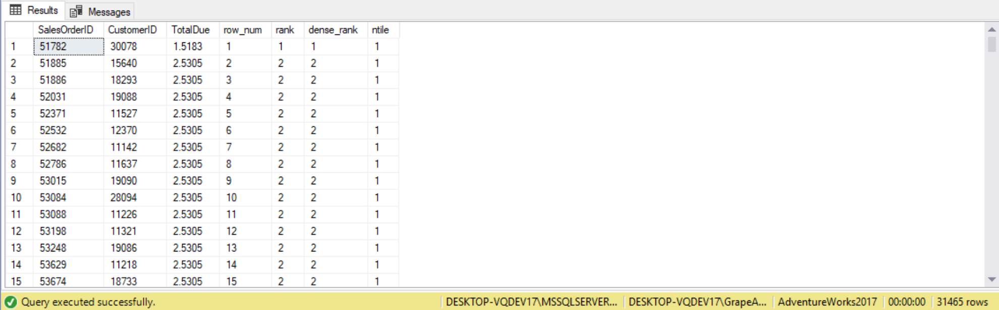
Ranking functions are used to rank each row with respect with the other rows in the window. If we specify the PARTITION BY clause with the RANK function, the ranking value will be restarted at 1 for every partition in the data set. There are four ranking functions in T-SQL: ROW_NUMBER, RANK, DENSE_RANK, and NTILE. The following query utilizes all four ranking functions, as shown below:
SELECT SalesOrderID,
       CustomerID,
       TotalDue,
       ROW_NUMBER() OVER(ORDER BY TotalDue) AS row_num,
       RANK() OVER(ORDER BY TotalDue) AS rank,
       DENSE_RANK() OVER(ORDER BY TotalDue) AS dense_rank,
       NTILE(100) OVER(ORDER BY TotalDue) AS ntile
FROM Sales.SalesOrderHeader;
ROW_NUMBER
There are times when we just want to generate a row number for each row in our output, where the row number is sequentially increased by 1 for each new row in the results set. To accomplish this, we can use the ROW_NUMBER function. The ROW_NUMBER function assigns unique, incremental sequential integers to rows within a respective partition based on a required window ordering. In our last query, we ORDER BY the val column, so as the value in the val column increases the row number does as well. Note that even if the value in the val column didn’t increase, the row number must still increase. So, if the ORDER BY attribute is not unqiue, the ROW_NUMBER query is nondeterministic, meaning more than one correct result is possible. For example, in our result set we have two instances of value 36.00, but one got a row number of 7 and the other 8. So any arrangement of those two row numbers would have been correct. To make the ROW_NUMBER query deterministic, we must add a tiebreaker to the ORDERBY list to make it unique, such as adding the orderid column.
The following query is an example of using the ROW_NUMBER function:
SELECT SalesOrderID,
       SalesOrderDetailID,
       LineTotal,
	   --No PARTITION BY clause
       ROW_NUMBER() OVER(ORDER BY SalesOrderID) AS RN,
       --With PARTITION BY clause
       ROW_NUMBER() OVER(PARTITION BY SalesOrderID ORDER BY SalesOrderDetailID) AS RN2
FROM Sales.SalesOrderDetail;
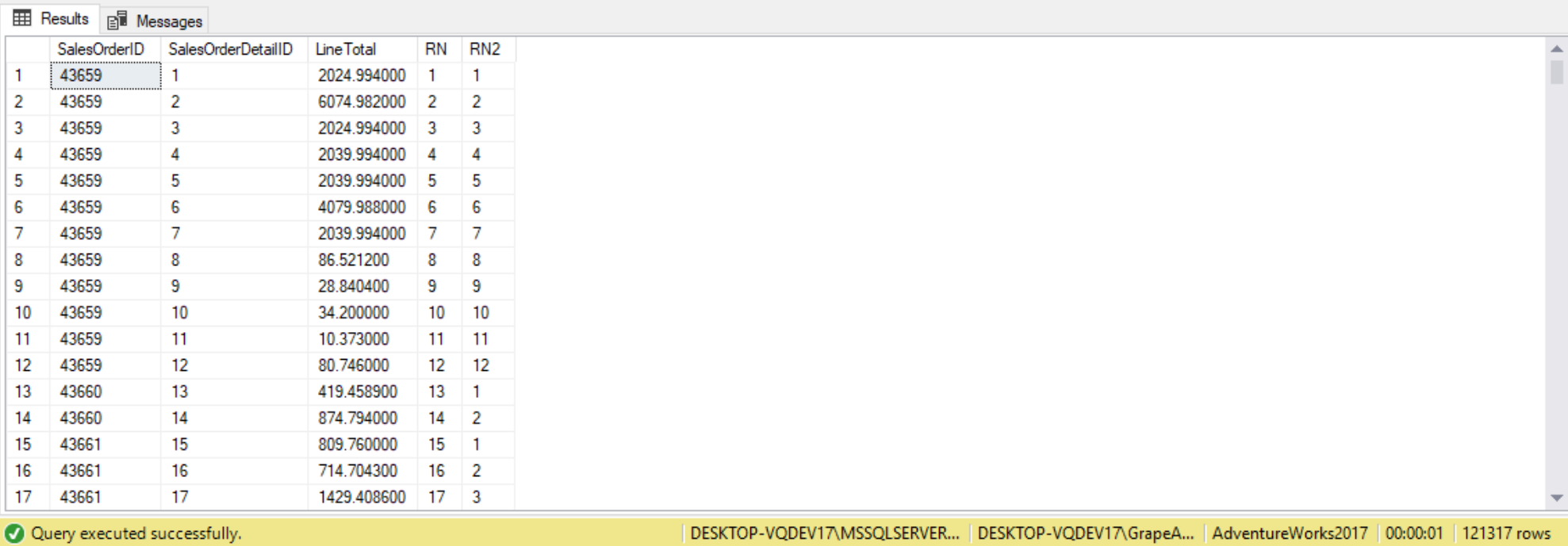
We can see each of the rows has a unique RowNumber column value. The RowNumber column values start at 1 and increments by 1 for each row. When we called the ROW_NUMBER() function we only specified the ORDER BY clause to order by the PostalCode column. Because we have no PARTITION BY clause the ROW_NUMBER() function returns a different RowNumber value for each row. Suppose we wanted to order the output by PostalCode, but we wanted the RowNumber to restart at 1 for each new StateProvinceID. To accomplish this, we add a PARTITION BY clause to my query, as follows:
As we can see, by adding the PARTITION BY clause to our query the RowNumber column value restarts at 1 for each new StateProvinceID value.
RANK:
The RANK function numbers each row in a partition sequentially starting at 1. A “partition” in a ranking function is a set of rows that have the same values for a specified partition column. If two rows in a partition have the same value for the ranking column (the column specified in the ORDER BY) then they will both get the same ranking value assignment.
As previously mentioned, ROW_NUMBER returns a nondeterministic result set when the ORDER BY attribute is not unique. To return the same rank value in the case of ties, we can use the RANK function. RANK reflects the count of rows that have a lower ordering value than the current row (plus 1).
The following query is a simple example of using the RANK function:
--RANK function vs ROW_NUMBER function
SELECT SalesOrderID,
       SalesOrderDetailID,
       LineTotal,
       --Rows in each partition are ranked by SalesOrderID ascending
       RANK() OVER(PARTITION BY SalesOrderID ORDER BY SalesOrderID) AS rank1,
       --Rows in each partition are ranked by LineTotal ascending
       RANK() OVER(PARTITION BY SalesOrderID ORDER BY LineTotal) AS rank2,
       ROW_NUMBER() OVER(PARTITION BY SalesOrderID ORDER BY SalesOrderDetailID) AS row_number
FROM Sales.SalesOrderDetail;

Difference between RANK() and ROW_NUMBER()is how RANK() deals with ties. Here in column rank2, there are two rows ranked 6, so the next rank is skipped to 8. Since there are three rows ranked 8, the next rank is 11. The ROW_NUMBER function will assign a unique number regardless.
The following is another example of using the RANK function:
USE AdventureWorks2012;
GO
SELECT PostalCode, StateProvinceID,
       RANK() OVER
         (PARTITION BY StateProvinceID
		  ORDER BY PostalCode ASC) AS RankingValue
FROM Person.Address
WHERE StateProvinceID IN (23,46);
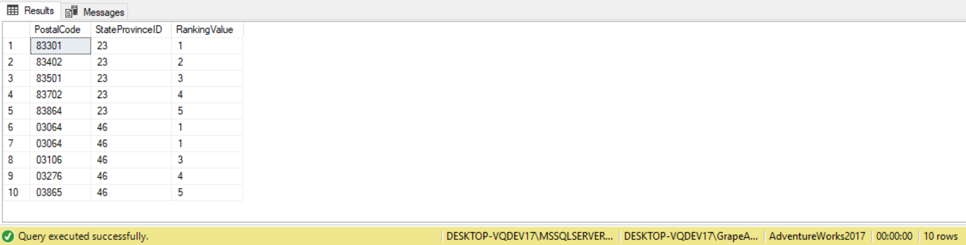
We can see the values created by the RANK function in the column RankingValue. In this example the ranking based on PostalCode. Each unique PostalCode gets a different ranking value. If we look at the rows of output for PostalCode 03054 you will see two rows, where each row has a RankingValue of 1. Because there were two PostalCode values of 03064,the RankingValue of 2 was skipped. The RankingValue for Postal Code 03106 then has a RankingValue of 3. The rest of the RankingValue data values were assigned the next sequential value because their PostalCode values where all unique. Since the PARTITION BY clause of the RANK function was not used in query above, the entire set was considered as a single partition. If we wanted to start the RankingValue over again for every unique StateProvinceID value all we would have to do is partition my results based on the StateProvinceID, as follows:
DENSE_RANK
What if we don’t wish for ranks to jump as in RNK column in the previous query. That’s where the DENSE_RANK() function comes in. DENSE_RANK() is the same as the RANK() function, only difference is that it will continue with the last rank evaluated and there is no gap.
--DENSE_RANK function vs. RANK function
SELECT SalesOrderID,
       SalesOrderDetailID,
       LineTotal,
       --Rows in each partition are ordered by LineTotal ascending
       RANK() OVER(PARTITION BY SalesOrderID ORDER BY LineTotal) AS RNK,
       DENSE_RANK() OVER(PARTITION BY SalesOrderID ORDER BY LineTotal) AS Dense_RNK
FROM Sales.SalesOrderDetail;

When we ran the RANK function for each duplicate PostalCode value, our output skipped a RankingValue. By using the DENSE_RANK function we can generate a ranking value that does not skip values. In other words, DENSE_RANK is similar to RANK, except it reflects the count of distinct
The only difference in syntax between the RANK function and the DENSE_RANK is the actual function name, as shown in an example query below:
(Include code, explanation, and results from SSC)
We see the rows with PostalCode 03064 have the same RankingValue, but the next PostalCode has a 2 instead of a 3. Recall the RANK function skipped a RankingValue for this same duplicate PostalCode. With DENSE_RANK it doesn’t skip a RankingValue when a duplicate PostalCode is found. Instead it keeps all the RankingValue sequential even when duplicate values are found.
NTILE
The NTILE function splits a set of records into groups. The number of groups returned is specified by an integer expression. It is used to associate rows in the result with tiles (equally sized groups of rows) by assigning a tile number to each row. We specify the number of tiles as well as the window ordering.
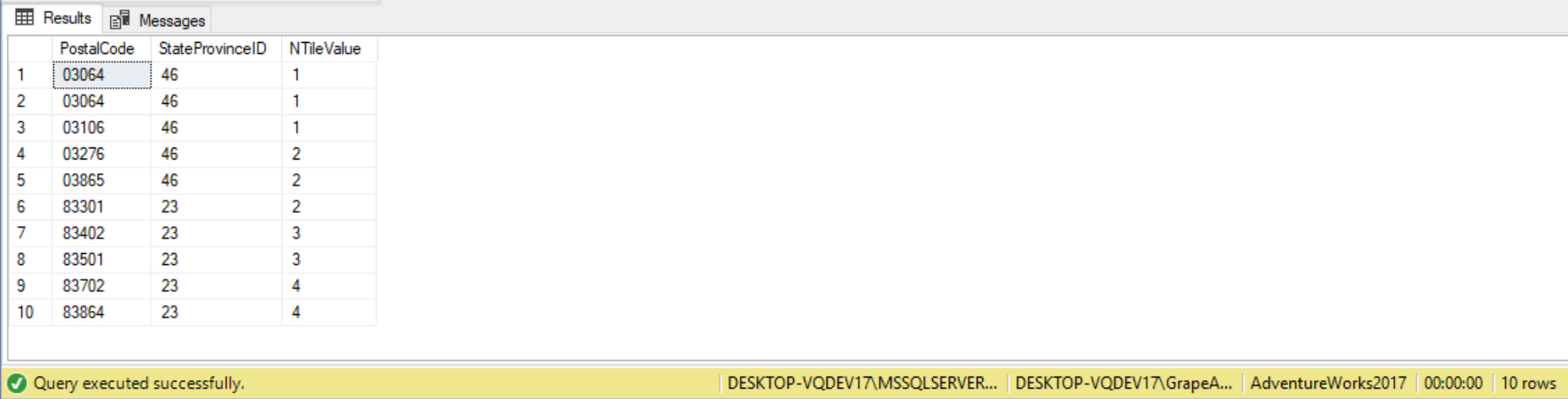
For the first example, suppose we want to put each PostalCode into one of two groups To accomplish meeting this we can run the NTILE function found in the query below:
SELECT PostalCode,
       StateProvinceID,
       NTILE(2) OVER(ORDER BY PostalCode ASC) AS NTileValue
FROM Person.Address
WHERE StateProvinceID IN(23, 46);

We can see that there are two different NTileValue column values: 1 and 2. The two different NTileValue values were created because we specified “NTILE(2)” in our SELECT statement. The value inside the parentheses following the NTILE function name is an integer expression, which specifies the number of groups that should be created. We see the query created two groups of rows as expected, with half the rows in each group. What happens when the set of records cannot be evenly divided by the NTILE integer_expression, causing a remainder? When this happens, one remainder row is placed in each group, starting from the first group, until all remainder rows have been assigned to a group. For example, if a table has 102 rows and 5 tiles were specified, the first 2 tiles will contain 21 rows instead of 20. The following query further illustrates how this works:
DECLARE @Integer_Expression INT= 4;
SELECT PostalCode,
       StateProvinceID,
       NTILE(@Integer_Expression) OVER(ORDER BY PostalCode ASC) AS NTileValue
FROM Person.Address
WHERE StateProvinceID IN(46, 23);
For example, our last query has 830 rows and we specified 10 tiles, so each tile has 83 tiles. The first tile (tile number 1) will contain the 83 lowest values from the val column specified in the ORDER BY, the next 83 are assigned tile number 2, and so on.
In the code above we defined a local variable named @Integer_Expression and assigned that variable a value of 4. This variable is then used in the call to NTILE function to specify returning 4 groups. We can see that SQL Server created 4 different groups. When we divide 10 by 4 you get a remainder of 2. This means that the first two groups should have 1 more row than the last two groups. In this output you can see that groups 1 and 2 each have 3 rows, whereas when the NTileValue is 3 and 4 there are only two rows associated with those groups.
Just like in the RANK function, we can also create NTILE ranking values within a partition by including the PARTITION BY clause in our NTILE function call. When we add the PARTITION BY clause SQL Server will start the NTILE ranking value at 1 for each new partition, like follows:
DECLARE @Integer_Expression int = 3;
SELECT PostalCode, StateProvinceID,
       NTILE(@Integer_Expression) OVER
		 (PARTITION BY StateProvinceID
		  ORDER BY PostalCode ASC) AS NTileValue
FROM Person.Address
WHERE StateProvinceID IN (46,23);
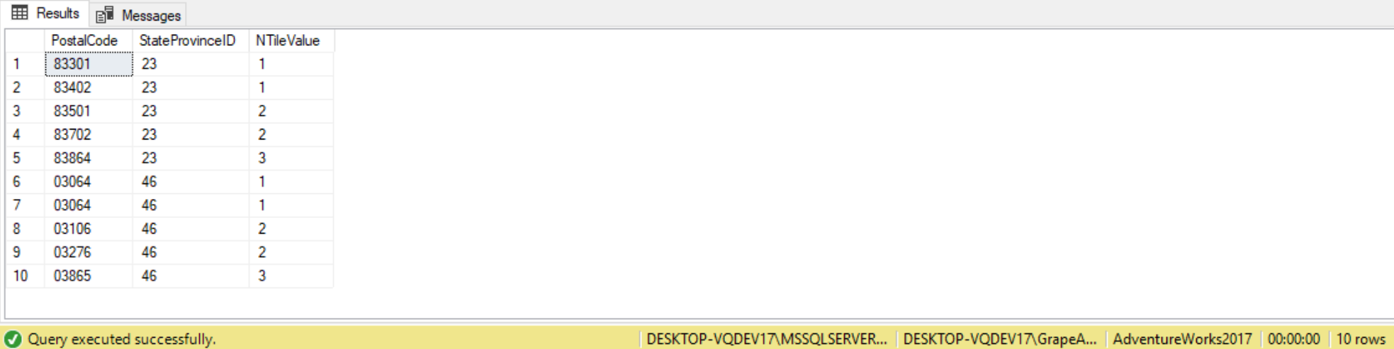
If we look at the column values for the output column NTileValue, we can see that the ranking values started over at 1 for the rows with a StateProvinceID value of 46. This was caused by adding the “PARTITION BY StateProvinceID” clause to our NTILE function specification.
Another example of the NTILE function:
--Subquery is evaluated before the NTILE function
SELECT SalesOrderID,
       SalesOrderDetailID,
       LineTotal,
       --Partition the data into 20 sets
       NTILE(4) OVER(ORDER BY SalesOrderID) AS NTILE2
FROM
(
    --NTILE function gets processed before the TOP function
    SELECT TOP (20) SalesOrderID,
                    SalesOrderDetailID,
                    LineTotal,
                    --Partition the data into 20 sets
                    NTILE(20) OVER(ORDER BY SalesOrderID) AS NTILE1
    FROM Sales.SalesOrderDetail
) AS SOH; --Always alias the subquery!

Offset/Analytical Window Functions
Analytical (or offset) window functions are used to return rows that are at a certain offset from the current row or at the beginning or end of a window frame. Analytical window functions supported by T-SQL include: LAG, LEAD, FIRST_VALUE, LAST_VALUE, CUME_DIST, PERCENTILE_CONT, PERCENTILE_DISC, PERCENT_RANK.
The LAG and LEAD functions are used to return an element from rows that is at a certain offset from the current row within the partition, based on the specified ordering. Both are supported by window partitions and window order clauses, and window framing have no relevance here. The LAG function looks before the current row, and the LEAD function looks ahead. The first argument is mandatory, and specifies the element we want to return. The second argument is optional, which specifies the offset (1 by default). A third argument is also optional, and specifies the default value to return if there is no row at the requested offset (NULL by default).
For example, the following query using the OrderValues view returns the previous order for each customer using LAG, and also the next order for each customer using LEAD:
(Include code, explanation, and results from page 242)
Since the query didn’t specify the offset or default value, the functions assumed an offset of 1 and the default value as NULL. To compute the difference between the current value and previous value of a customer’s order using val-LAG(val) OVER(…). We can also compute the difference between the current and next values using val-LEAD(val) OVER(…).
The code to create our demo table is as follows:
--Drop table if it already exists
IF OBJECT_ID('dbo.MicrosoftStockHistory') IS NOT NULL
DROP TABLE dbo.MicrosoftStockHistory;
GO
--Creating table dbo.MicrosoftStockHistory
SET ANSI_NULLS ON;
GO
CREATE TABLE dbo.MicrosoftStockHistory
([Date]     DATE NOT NULL,
 OpenPrice  NUMERIC(5, 2) NOT NULL,
 High       NUMERIC(5, 2) NOT NULL,
 Low        NUMERIC(5, 2) NOT NULL,
 ClosePrice NUMERIC(5, 2) NOT NULL,
 Volume     BIGINT NOT NULL,
 AdjClose   NUMERIC(5, 2) NOT NULL
)
ON [Primary];
GO
--Load Table using Bulk Intert
BULK INSERT MicrosoftStockHistory FROM 'C:\Users\GrapeApe561\Desktop\Microsoft Stock Info.csv' WITH(FIRSTROW = 2, --First row of table is second row on the csv
FIELDTERMINATOR = ',', --CSV field delimiter
ROWTERMINATOR = '\n', --Use to shift the control to next row
TABLOCK); --Table lock to make the bulk insert a bit quicker

SELECT * FROM dbo.MicrosoftStockHistory;
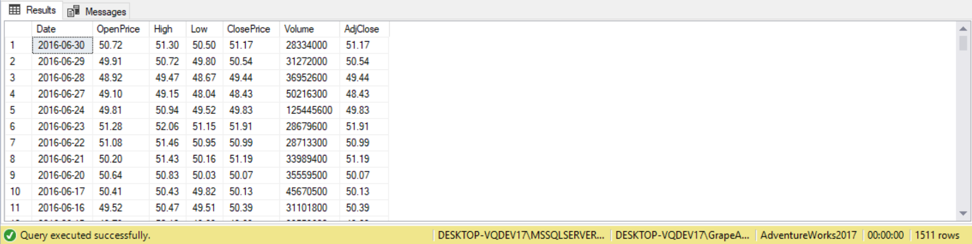
What is the change in ClosePrice from one day to the next? What if we have a 3 day weekend like from 7/2/10 to 7/6/10?
SET STATISTICS IO ON;
SELECT *,
       --Bring close price for Month-Year(first day)
       --Using the default of RANGE, so it not using memory
       FIRST_VALUE(ClosePrice) OVER(PARTITION BY MONTH(date),
                                                 YEAR(date) ORDER BY [Date] ROWS UNBOUNDED PRECEDING) AS BeginClosePrice, --Improve performance using framing
       --End close price for Month-Year(last day). Unbounded Preceding to current row
       --All preceding rows in that partition to current row
       LAST_VALUE(ClosePrice) OVER(PARTITION BY MONTH(date),
                                                YEAR(date) ORDER BY date) AS EndClosePrice,
       --Same query as last the above LAST_VALUE query, but using framing
       LAST_VALUE(ClosePrice) OVER(PARTITION BY MONTH(date),
                                                YEAR(date) ORDER BY [Date] ROWS BETWEEN CURRENT ROW AND UNBOUNDED FOLLOWING) AS Real_EndClose
--All the way till end of partition. This query is forced into memory
FROM dbo.MicrosoftStockHistory;
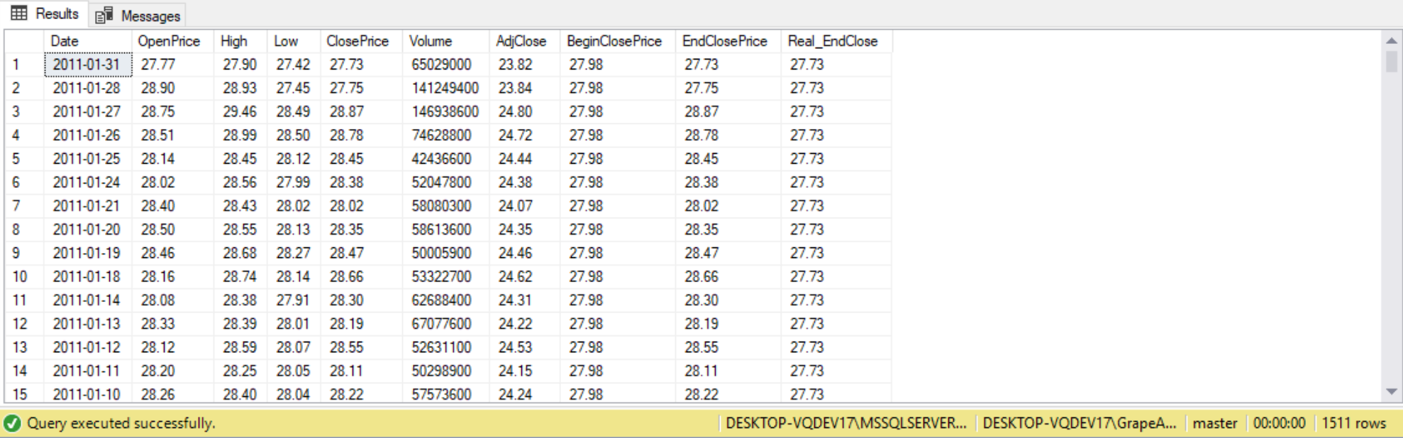
^^ Scan count and logical reads should be 0. See why this didn’t happen.
/* === Questions ===
1.) What is the difference between my previous day close?
a.) First Method: Use self join
b.) Second method: Use ROW_NUMBER and self join in a CTE
c.) Third method: Use LAG function
2.) How many days has the price dropped in a row?
*/
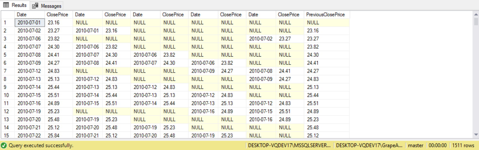
SET STATISTICS IO, TIME ON;
--Method 1: Self Join
SELECT m1.Date, --Current date
m1.ClosePrice,
m2.Date, --Previous date
m2.ClosePrice,
m3.Date,
m3.ClosePrice,
m4.Date,
m4.ClosePrice,
m5.Date,
m5.ClosePrice,
COALESCE(m2.ClosePrice, m3.ClosePrice, m4.ClosePrice, m5.ClosePrice) AS PreviousClosePrice
FROM dbo.MicrosoftStockHistory AS m1
LEFT JOIN dbo.MicrosoftStockHistory AS m2 ON m1.Date = DATEADD(dd, 1, m2.Date)
LEFT JOIN dbo.MicrosoftStockHistory AS m3 ON m1.Date = DATEADD(dd, 2, m3.Date) --Maybe holiday
LEFT JOIN dbo.MicrosoftStockHistory AS m4 ON m1.date = DATEADD(dd, 3, m4.Date) --Maybe Weekend
LEFT JOIN dbo.MicrosoftStockHistory AS m5 ON m1.Date = DATEADD(dd, 4, m5.Date) --Maybe weekend and holiday
ORDER BY m1.Date;
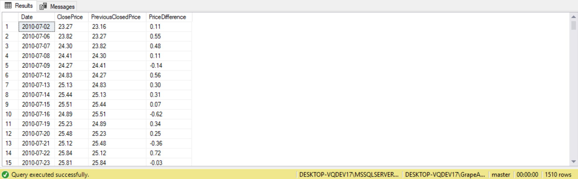
SET STATISTICS IO, TIME ON;
--Method 2: Using ROW_NUM and self join in a CTE
WITH PreviousDay
     AS (SELECT Date,
                ClosePrice,
                ROW_NUMBER() OVER(PARTITION BY 1 ORDER BY date) AS RN
         FROM dbo.MicrosoftStockHistory)
     SELECT p1.Date,
            p1.ClosePrice,
            p2.ClosePrice AS PreviousClosedPrice,
            p1.ClosePrice - p2.ClosePrice AS PriceDifference
     FROM PreviousDay AS p1
          JOIN PreviousDay AS p2 ON p1.RN = p2.RN + 1; --'+' goes back 1 row
SET STATISTICS IO, TIME ON;
--Method 3: LAG/LEAD
SELECT Date,
       ClosePrice,
       --Goes back one record. Here it is going one day back for ClosePrice
       LAG(ClosePrice) OVER(ORDER BY Date) AS PreviousDayClose,
       --Difference in ClosePrice between current date and previous date
       ClosePrice - (LAG(ClosePrice) OVER(ORDER BY Date)) AS Diff
FROM dbo.MicrosoftStockHistory;
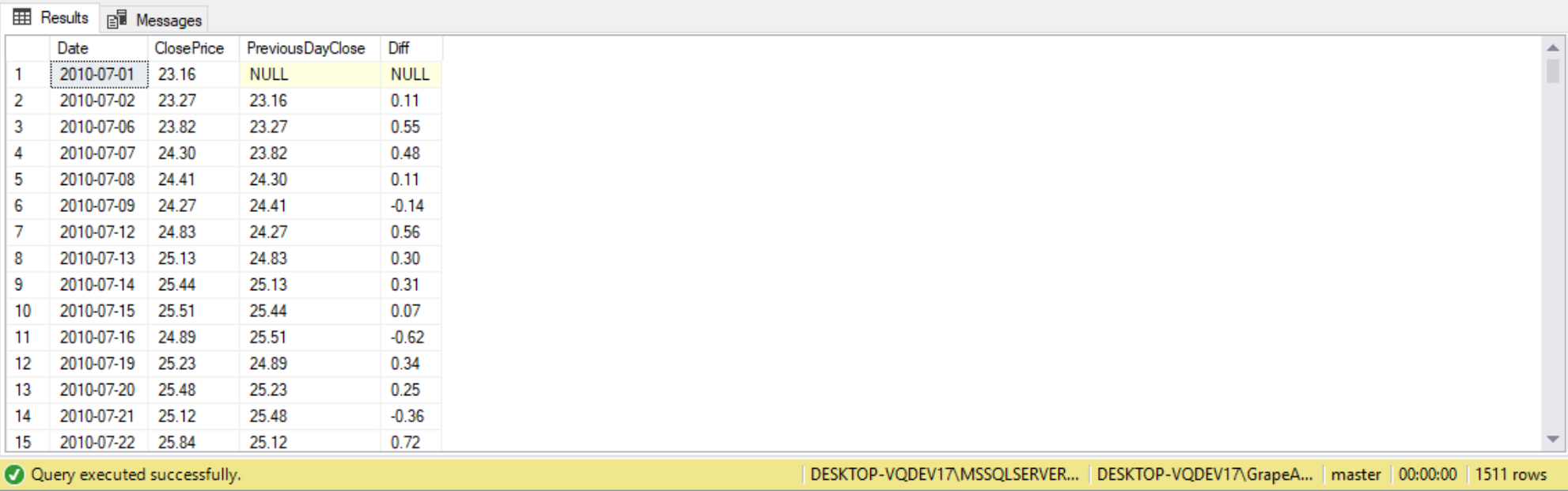
There will be no NULLs besides for the first row. Regardless of how big the gap is between the dates, the LAG function is going to go simply back one row in the result set (for date) and get that value for ClosePrice.
As we can see from the statics io and time, the third method (LAG/LEAD) is the quickest method out of the three we executed:

The FIRST_VALUE and LAST_VALUE functions return the elements from the first and last row in the window frame, respectively. These functions are supported by window-partition, window-order, and the window frame clauses. To return the element from the first row of the window partition, we use FIRST_VALUE with a specified window frame extent ROWS BETWEEN UNBOUNDED PRECEDING AND CURRENT ROW. To return an element from the last row in the window partition, we use LAST VALUE with the window frame extent ROWS BETWEEN CURRENT ROW AND UNBOUNDED FOLLOWING. If we specify the ORDER BY clause without a window-frame unit (such as ROWS), the bottom delimiter will be CURRENT ROW by default, which is not what we want when using LAST_VALUE. For performance-related reasons, it is best practice to be explicit about the window-frame extent even for FIRST_VALUE.
For example, the following query uses the FIRST_VALUE function to return the value of the customers first order and the LAST_VALUE function to return the value of the customer’s last order:
(Include code, explanation, and results from page 243)
To compute the difference between the customer’s current and first order values, we can write val-FIRST_VALUE(val) OVER(…). Similarly, to compute the difference between the customer’s current and last order values, we can write val-LAST_VALUE(val) OVER(…).
(Include code from Pragmatic Works)
Aggregate window functions
Window Functions allow us to add aggregate calculations to non-aggregate queries. Aggregate window functions are used to aggregate the rows in a defined window. They are supported by window-partition, window-order, and window-frame clauses.
Remember an OVER clause with empty parentheses sets the window to include all rows from the underlying query’s result set to the function. For example, SUM(val) OVER() returns the grand total of all the query’s entire result set. By using a window-partition clause, we apply the function restricted by window. For example, SUM(val) OVER(PARTITION BY custid) returns the total values for the current customer.
The query below uses the OrderValues view, and returns along with each order, the grand total of all order values as well as the customer total:
(Include code, explanation, and results from page 244)
The totalvalue column shows the grand total for all values, whereas the custtotalvalue shows the total values for the current customer.
As an example of mixing details an aggregates with window functions, the following query calculates for each row the percentage of the current value out of the grand total, as well as the customer total:
(Include code, explanation, and results from page 245)
Aggregate window functions also support a window frame, which allows for more sophisticated calculations such as running and moving aggregates, YTD and MTD calculations.
Using window functions we can write an aggregate query with no GROUP BY, and yet we can immediately show the totals for the entire result set, or specific partitions we have added into the result set.
--Window functions: SUM()
SELECT SalesOrderID,
       SalesOrderDetailID,
       LineTotal,
       --Total LineTotal for all sales
       sum(LineTotal) OVER() AS WithoutPartitionBy,
       --Subquery that does the same thing as the about SUM() window function
(
    SELECT SUM(LineTotal)
    FROM Sales.SalesOrderDetail
) AS Alternative,
       --Partitioned By SalesOrderID
       sum(LineTotal) OVER(PARTITION BY SalesOrderID) AS SOID_Partition,
       --Percent of Total for each SalesOrderID
       LineTotal / SUM(LineTotal) OVER(PARTITION BY SalesOrderID) * 100 AS PercentOfTotal
FROM Sales.SalesOrderDetail;

Note that the SUM() Window function with PARTITION BY may perform worse compared to using a CTE or a correlated subquery.
For example, suppose our goal is to calculate a running total that resets whenever the TransactionDate changes. We’ll total the TransactionAmount. For each subsequent invoice within the transaction date, the RunningTotal should equal the prior InvoiceID’s running total plus the current TransactionAmount. The query would be as follows:
(Include code, explanation, and results from Wenzel)
Notice there is no GROUP BY clause. This is surprising, typically aggregate functions, such as SUM, require a GROUP BY clause; so why is this the case? With GROUP BY we need to specify each column in the SELECT clause that isn’t an aggregate function. Since we are using the OVER…PARTITION BY clause, the SUM is considered a window function – it operates upon any rows defined in the OVER clause. We PARTITION BY TransactionDate, meaning that the SUM operates on all rows with the same TransactionDate. This defines the window of rows the SUM function affects.
Up to this point we have partitioned the data and are able calculate a subtotal for all TransactionAmount values within a TransactionDate. The next step is to now calculate the subtotal. To do this we can use ORDER BY within the OVER clause to define the “scope” of the window function. The ORDER BY specified the logical order the window function operates.
(Include code, explanation, and results from Wenzel)
The difference between this window function and that from the first step, is ORDER BY InvoiceID. This specifies the logical order to process within the partition. Without the ORDER BY the logical order is to wait until we are at the end of the window to calculate the sum. With the ORDER BY specified, the logical order is to calculate a sum for each row including previous TransactionAmount values within the window.
Note that we could have calculated the same running totals using an INNER JOIN, but window functions are superior in terms of performance.
(Include code, explanation, and QUERY PLAN FOR BOTH QUERIES from Wenzel)
For example:
(Include code, explanation, and results from page 246)
Window Framing
A window frame clause filters the subset of rows from the window partition between two specified delimiters. These allow us to specify a range of rows that are used to perform the calculations for the current row. Two window-frame units include ROWS and RANGE. ROWS specifies the window using rows, and RANGE specifies the window as a logical offset.
Aggregate window functions also support a window frame, which allows for more sophisticated calculations such as running and moving aggregates, YTD and MTD calculations.
ROWS/RANGE are always used inside the OVER() clause to limit the records within the PARTITION BY. The PARTITION BY takes in a result set and essentially limits that result set by the partition. The rows in the RANGE clause allows us to further limit those records within the PARTITION BY, and we can specify the start and the end of the partition per row. Range is the default behavior which will use the TempDB. TempDB is going to be using disc on our computer or server.
ROWS is going to use Memory, and will typically perform better. But in order to use memory, we have to explicitly say in our code that you want to use ROWS.
Preceding: We want to get rows that are preceding the current row. 1 preceding goes back one row, whereas unbounded preceding goes all the way back to the beginning of the partition that we’re currently in.
Framing in window functions will only work when we use the ORDER BY clause. That’s why totals will sometimes work better with older and more complex T-SQL methods because we can’t use framing to actually improve the performance there.
(Include codes from Pragmatic Works)
Windows Spool can be found in the execution plan whenever we’re using tempdb or memory. Unfortunately, the execution plan itself, when seeing Windows Spool, will not let us know whether it’s using specifically tempdb or memory. In order to find this out, we would have to look into the STATISTICS IO. Table Spool uses disc and also tempdb.
When go in STATISTICS IO and look at the messages, we wanna look at the work table there and see the total scan count. A scan count of 0 means the worktable and tempdb was not used. A scan count greater than 0 means that the work table created in tempdb was used, and the tempdb was used on disc.
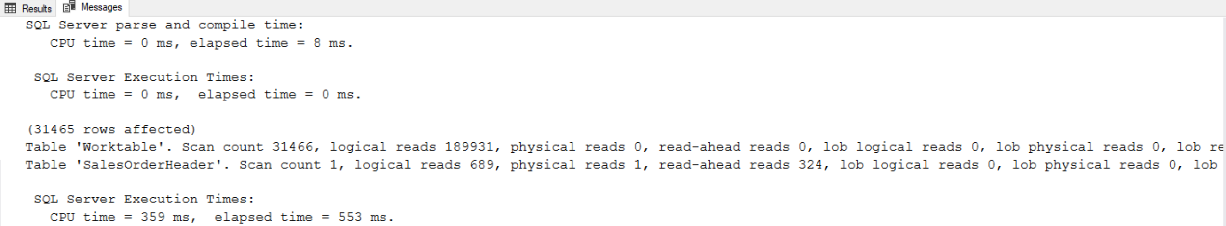
SET STATISTICS IO, TIME ON;
SELECT CustomerID,
       SalesOrderID,
       OrderDate,
       TotalDue,
       --Using default of RANGE, which is going to use tempdb
       SUM(TotalDue) OVER(ORDER BY SalesOrderID RANGE UNBOUNDED PRECEDING) AS RunningTotal
FROM Sales.SalesOrderHeader;

SELECT CustomerID,
       SalesOrderID,
       OrderDate,
       TotalDue,
       --Using ROWS, which is going to use memory
       SUM(TotalDue) OVER(ORDER BY SalesOrderID ROWS UNBOUNDED PRECEDING) AS RunningTotal2
FROM Sales.SalesOrderHeader;

Using the default of RANGE in the first query, we get a scan count of greater than 0, so we know it’s using tempdb. In the second query worktable and tempdb was NOT used (since the scan count is 0), so the query did use memory:
The following code serves as proof that RANGE UNBOUNDED PRECEDING is the default behavior:
SET STATISTICS IO, TIME ON;
SELECT CustomerID,
       SalesOrderID,
       OrderDate,
       TotalDue,
       --Using default of RANGE, which is going to use tempdb
       SUM(TotalDue) OVER(ORDER BY SalesOrderID) AS RunningTotal
FROM Sales.SalesOrderHeader;
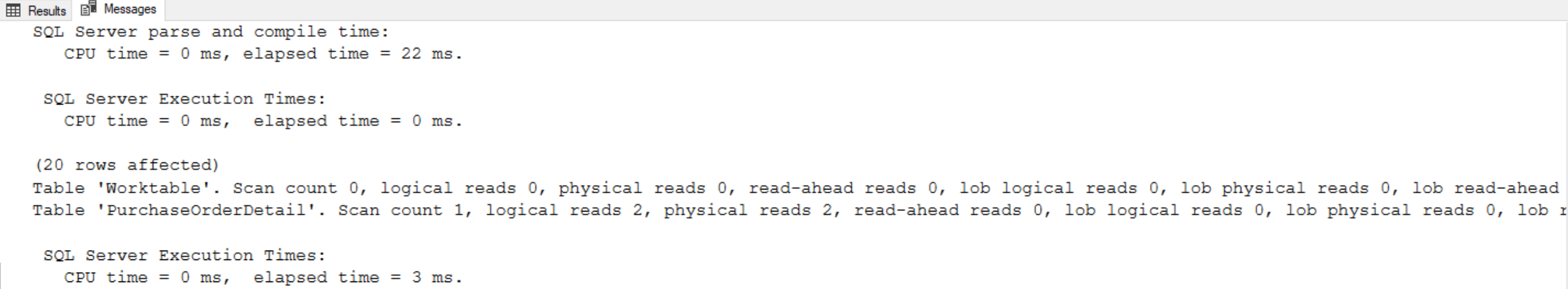
The query below is one more example of using the ROWS window frame. Because we’re using ROWS, we will see the worktable scan count is 0, so we know it’s using memory:
SET STATISTICS IO ON;
SELECT PurchaseOrderID,
       PurchaseOrderDetailID,
       ProductID,
       LineTotal,
       --No partion, so entire result set
       SUM(LineTotal) OVER(ORDER BY PurchaseOrderID
	                  ROWS BETWEEN CURRENT ROW AND UNBOUNDED FOLLOWING) AS RunningTotal,
       --Partition by PurchaseOrderID
       SUM(LineTotal) OVER(PARTITION BY PurchaseOrderID ORDER BY PurchaseOrderID
					  ROWS BETWEEN CURRENT ROW AND UNBOUNDED FOLLOWING) AS RunningTotalBy_PurchaseOrder
FROM Purchasing.PurchaseOrderDetail
WHERE PurchaseOrderID < 10
ORDER BY PurchaseOrderID,
         PurchaseOrderDetailID;
The following code queries running totals for three line items, see the highlighted cells to see what cells were added to get running total:
SET STATISTICS IO ON;
SELECT PurchaseOrderID,
       PurchaseOrderDetailID,
       ProductID,
       LineTotal,
       --Running Total for 3 line items
       SUM(LineTotal) OVER(ORDER BY PurchaseOrderID
		ROWS BETWEEN 1 PRECEDING AND 1 FOLLOWING) AS RunningTotal
FROM Purchasing.PurchaseOrderDetail
WHERE PurchaseOrderID < 10
ORDER BY PurchaseOrderID,
         PurchaseOrderDetailID;

Range can only be used with UNBOUNDED preceding or UNBOUNDED following. We cannot hard coded values like 2 following or 1 preceding for RANGE:
SET STATISTICS IO ON;
SELECT PurchaseOrderID,
       PurchaseOrderDetailID,
       ProductID,
       LineTotal,
       --Running Total for 3 line items
       SUM(LineTotal) OVER(ORDER BY PurchaseOrderID
	   RANGE BETWEEN 1 PRECEDING AND 2 FOLLOWING) AS RunningTotal
FROM Purchasing.PurchaseOrderDetail
WHERE PurchaseOrderID < 10
ORDER BY PurchaseOrderID,
         PurchaseOrderDetailID;

RANGE can give us different results, especially when doing running totals with the ORDER BY clause. Explanation around 22:00 mark:
--Running Total using RANGE vs. ROWS
SELECT SalesOrderID,
       SalesOrderDetailID,
       LineTotal,
       SUM(LineTotal) OVER(PARTITION BY SalesOrderID ORDER BY LineTotal) AS RunningTotal_Range,
       SUM(LineTotal) OVER(PARTITION BY SalesOrderID ORDER BY LineTotal ROWS UNBOUNDED PRECEDING) AS RunningTotal_Rows
FROM Sales.SalesOrderDetail;

^^Using the Rows method. Notice the duplicates in line 6 and 7. Around 24:00 mark.
(Include code from Wenzel)
The above query returns for each employee and month the monthly value, as well as the running totals from the beginning of the employees’ activity until the current month. We partition the window by empid to apply the calculation to each employee independently, then define the ordering by ordermonth, and specify the window framing as ROWS BETWEEN UNBOUNDED PRECEEDING AND CURRENT (which means all activity from the beginning of the partition until the current month).
Delimiters used in conjunction with ROWS window-frame unit include: PRECEDING, FOLLOWING, UNBOUNDED, and CURRENT. With PRECEDING, we want to get rows that are preceding the current row. 1 preceding goes back one row, whereas unbounded preceding goes all the way back to the beginning of the partition that we’re currently in. We can indicate an offset back or offset forward from the current row. For example, to capture all rows from two rows before the current row until one row ahead, we can specify ROW BETWEEN 2 PRECEEDING AND 1 FOLLOWING. Also, if we don’t want an upper bound, we can specify UNBOUNDED FOLLOWING.
Alternative Methods to Window Functions
There are alternative methods available to solve the same problems that we’ve solved with window functions. For example, how can we get running totals without using window functions, and how will the alternative methods impact performance? And how maintainable is this code going to be?
For calculating running totals, using window functions is not only the cleanest method as far as the amount of code we have to write and how easy it is to read that code, but it’s also the best performing option we have here as well.
SET STATISTICS IO ON;

--Running Total using window function
SELECT CustomerID,
       SalesOrderID,
       OrderDate,
       TotalDue,
       SUM(TotalDue) OVER(PARTITION BY CustomerID ORDER BY SalesOrderID
	                 ROWS BETWEEN UNBOUNDED PRECEDING AND CURRENT ROW) AS RunningTotal
FROM Sales.SalesOrderHeader;

Notice that the worktable is not being used (0 scan count), so we forced it into memory. Also notice the SalesOrderTable table is being scanned only one time here. This is the functionality we get from the window function: the main table is being scanned one time and it’s doing everything in memory.
SET STATISTICS IO ON;

--Running Total using correlated subquery
SELECT CustomerID,
       SalesOrderID,
       OrderDate,
       TotalDue,
(
    SELECT SUM(TotalDue)
    FROM Sales.SalesOrderHeader
    WHERE CustomerID = a.CustomerID
          AND SalesOrderID <= a.SalesOrderID
) AS RunningTotal
FROM Sales.SalesOrderHeader AS a;

Notice that we are using the worktable, so tempdb is being used here. Notice also that we had to scan the SalesOrderHeader table 2 times. This is a problem that happens a lot with correlated subqueries. If we added another correlated subquery for MIN() and then for MAX(), the scan count will increase 1 time for each one, so the performance gets worse and worse as we continue to add additional aggregations to the correlated subquery.
SET STATISTICS IO ON;

--Running Total using self join
SELECT a.CustomerID,
       a.SalesOrderID,
       a.OrderDate,
       a.TotalDue,
       SUM(b.TotalDue)
FROM Sales.SalesOrderHeader AS a
     JOIN Sales.SalesOrderHeader AS b ON a.CustomerID = b.CustomerID
                                         AND a.SalesOrderID >= b.CustomerID
GROUP BY a.CustomerID,
         a.SalesOrderID,
         a.OrderDate,
         a.TotalDue
ORDER BY CustomerID,
         SalesOrderID;

Because we’re doing a self-join, we’re querying the data two times, once again the table is being scanned twice, meaning more overhead. As the table grows in size, the performance is going to get significantly worse using these methods.
As we can see, window functions perform nore efficiently compared to the older, more complex methods that we have available.
Generally window functions will yield the best performance but in the following example RANGE the default frame delimiter is used and therefore work is done on disk. CTEs will perform the best here because the work will be done in memory.
(Include rest of content from Pragmatic Works)
SET STATISTICS IO, TIME ON;

--Window Aggregate Function Method: 1 aggregate function in this query
SELECT SalesOrderID,
       SalesOrderDetailID,
       LineTotal,
       SUM(LineTotal) OVER(PARTITION BY SalesOrderID) AS TransactionTotal
FROM Sales.SalesOrderDetail;

--Window Aggregate Function Method: 3 aggregate functions in this query
SELECT SalesOrderID,
       SalesOrderDetailID,
       LineTotal,
       SUM(LineTotal) OVER(PARTITION BY SalesOrderID) AS TransactionTotal,
       MIN(LineTotal) OVER(PARTITION BY SalesOrderID) AS MinTotal,
       MAX(LineTotal) OVER(PARTITION BY SalesOrderID) AS MaxTotal
FROM Sales.SalesOrderDetail;
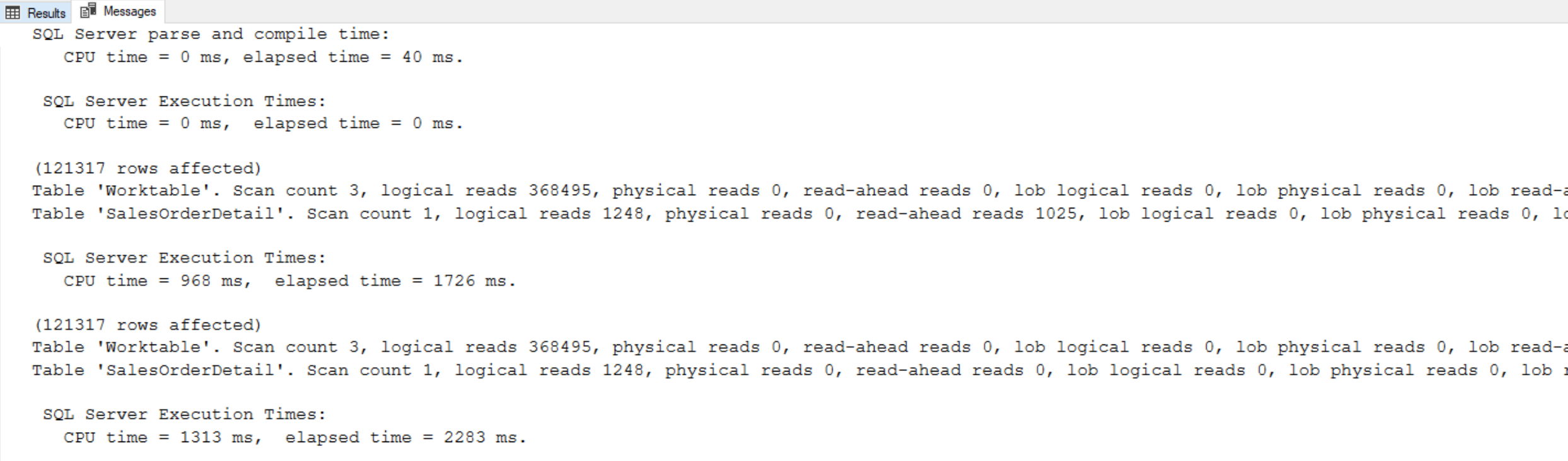
This query is using tempdb. It is using RANGE, which is the default behavior. Remember, framing only works if we use an ORDER BY clause. Whenever we’re doing totals, we cannot add an ORDER BY clause because if we add an ORDER BY clause, it turns into a running total. Since we cannot use framing, we cannot use ROWS and we cannot force this into memory. Notice that the query above has worktable scan count of 3 and logical reads of 368495, and the table itself was scanned 1 time. This is one of those cases where the window functions may not perform the best.
As we can see from the two queries in the code box above, when adding additional aggregates the performance impact is minimal as long as we’re using the same OVER clause (ie. same window).
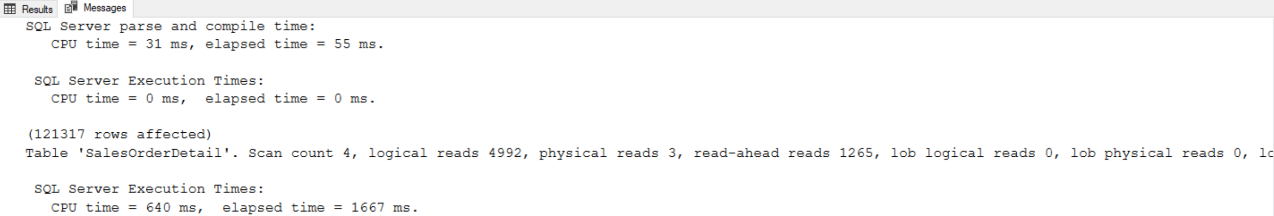
Let see how the performance compares using a CTE:
SET STATISTICS IO, TIME ON;

--CTE Method
WITH Totals
     AS (SELECT SalesOrderID,
                SUM(LineTotal) AS Total,
                MIN(LineTotal) AS MinTotal,
                MAX(LineTotal) AS MaxTotal
         FROM Sales.SalesOrderDetail
         GROUP BY SalesOrderID)
     SELECT sod.SalesOrderDetailID,
            sod.SalesOrderID,
            sod.LineTotal
     FROM Sales.SalesOrderDetail AS sod
          JOIN Totals AS t ON sod.SalesOrderID = t.SalesOrderID;

Notice in the above query that we are scanning the table twice, but we only have 2496 logical reads. Overall, this query will perform significantly better, especially as we get more and more records that we’re trying to run the T-SQL query against.
Let see how the performance compares when we use a correlated subquery:
SET STATISTICS IO, TIME ON;

--Correlated subquery method
SELECT SalesOrderID,
       SalesOrderDetailID,
       LineTotal,
(
    SELECT SUM(LineTotal)
    FROM Sales.SalesOrderDetail
    WHERE SalesOrderID = sod.SalesOrderID
) AS Total,
(
    SELECT MIN(LineTotal)
    FROM Sales.SalesOrderDetail
    WHERE SalesOrderID = sod.SalesOrderID
) AS MinTotal,
(
    SELECT MAX(LineTotal)
    FROM Sales.SalesOrderDetail
    WHERE SalesOrderID = sod.SalesOrderID
)
FROM Sales.SalesOrderDetail AS sod;
As we can see, performance will go down as additional aggregations are added here. The table will need to be scanned additional times proportionate to the number of aggregates needed. Notice the correlated subquery has 3 aggregations. Every time we add an aggregation and a correlated subquery, it has to scan that base table. So with 3 aggregations plus the default behavior (which is scanning the table for SalesOrderID), we get a scan count of 4. So the performance of the correlated subquery is going to get worse and worse as you add additional aggregations, because it has to go back and scan that base table for each correlated subquery.
So generally speaking, when doing totals, your best option for performance is going to working the context of a CTE, and then correlated subqueries, and then going back to the window function itself (VERIFY THIS BY RE-DOING above codes).