Inserting data

• The INSERT VALUES statement
• The INSERT SELECT statement
• The SELECT INTO statement
• The BULK INSERT statement

The identity property and the sequence object

• Identity
• Sequence

Deleting data

• The DELETE statement
• The TRUNCATE statement
• DELETE based on a join

Updating Data

• The UPDATE statement
• UPDATE based on a join
• Assignment UPDATE

Merging data

Modifying data through table expressions

Modifications with TOP and OFFSET-FETCH

The OUTPUT clause

• INSERT with OUTPUT
• DELETE with OUTPUT
• UPDATE with OUTPUT
• MERGE with OUTPUT
• Nested DML

Inserting data

DML involves not only data modification, but also data retrieval. DML statements include: SELECT, INSERT, UPDATE, DELETE, TRUNCATE, and MERGE.

T-SQL statements for inserting data into tables include: INSERT VALUES, INSERT SELECT, INSERT EXEC, SELECT INTO, and BULK INSERT.

The INSERT VALUES statement

The standard INSERT VALUES statement is used to insert rows into a table based on specified values. The following code :

USE AdventureWorks2017;
DROP TABLE IF EXISTS dbo.Orders;
CREATE TABLE dbo.Orders
(SalesOrderID  INT NOT NULL
                   CONSTRAINT PK_Orders PRIMARY KEY, 
 OrderDate     DATE NOT NULL
                    CONSTRAINT DFT_orderdate DEFAULT(SYSDATETIME()), 
 SalesPersonID INT NOT NULL, 
 CustomerID    VARCHAR(10) NOT NULL
);

While specifying the target column names right after the table name is optional, it is good practice because we can control the value-column associations instead of relying on the order of the columns in the CREATE TABLE statement. In T-SQL, specifying the INTO clause is also optional.

If we don’t specify a value for a column, SQL Server will use any default value defined for the column. If there is no default value defined and the column allows NULLs, then NULL will be used. If no default is specified and the column does not accept NULLs, our INSERT statement will fail.

T-SQL supports an enhanced standard VALUES clause we can use to specify multiple rows separated by commas. For example, the following statement inserts four rows into the Orders table:

INSERT INTO dbo.Orders(SalesOrderID,OrderDate,SalesPersonID,CustomerID)
VALUES
(10003,'20160213',4,'B'),
(10004,'20160214',1,'A'),
(10005,'20160213',1,'C'),
(10006,'20160215',3,'C');

This statement processed as a transaction, meaning that if any row fails to enter the table, none of the rows in the statement enters the table. We can also use the enhanced VALUES clause as a table-value constructor to construct a derived table. For example:

SELECT * FROM 
(VALUES
(10003,'20160213',4,'B'),
(10004,'20160214',1,'A'),
(10005,'20160213',1,'C'),
(10006,'20160215',3,'C')) 
AS o(SalesOrderID,OrderDate,SalesPersonID,CustomerID);

Following the parentheses that contain the table value constructor, we assign an alias to the table (O in this case), and following the table alias we assign aliases to the target columns in parentheses.

The INSERT SELECT statement

The standard INSERT SELECT statement inserts a set of rows returned by a SELECT query into a target table. The syntax is similar to the INSERT VALUES statement, but instead of the VALUES keyword we specify a SELECT query. For example, the following code inserts into the dbo.Orders table the result of a query against the Sales.Orders table and returns orders that were shipped to the United Kingdom:

INSERT INTO dbo.Orders
(SalesOrderID, 
 OrderDate, 
 SalesPersonID, 
 CustomerID
)
       SELECT SalesOrderID, 
              OrderDate, 
              SalesPersonID, 
              CustomerID
       FROM Sales.SalesOrderHeader
       WHERE TerritoryID = '4'
             AND SalesPersonID IS NOT NULL;
SELECT * FROM dbo.Orders;

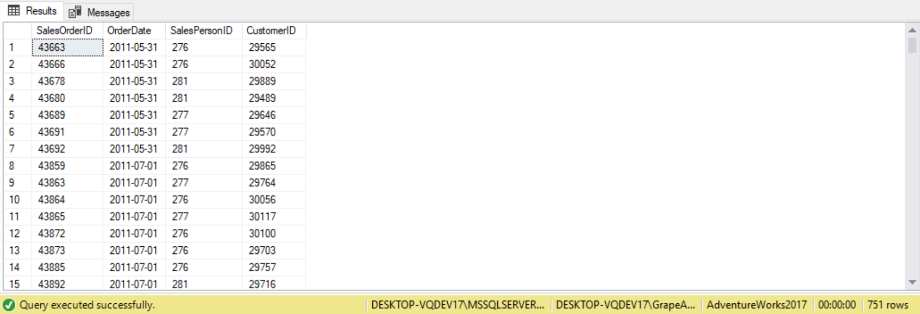
The INSERT SELECT statement can also be used to specify the target column names, which is best practice. The behavior in terms of relying on a default constraint or column nullability is also the same as with the INSERT VALUES statement. The INSERT SELECT statement is also performed as a transaction, so if any row fails to enter the target table, none of the rows enter the table. (Note that is we include a system function such as SYSDATETIME in the inserted query, the function gets invoked only once for the entire query and not once per row. The exception to this rule is if we generate globally unique identifiers (GUIDs) using the NEWID function, which gets invoked per row).

The INSERT EXEC statement

The INSERT EXEC statement can be used to insert a result set from a stored procedure or a dynamic SQL batch into a target table. The INSERT EXEC statement is similar in syntax and concept to the INSERT SELECT statement, but instead of the SELECT statement we specify the EXEC statement. For example, the following code creates a stored procedure called Sales.GetOrders, and it returns orders that were shipped to a specified input country (with the @country parameter).

(Include code from page 273)

The SELECT INTO statement

The SELECT INTO statement is nonstandard and exclusive to T-SQL. It creates a target table and populates it with the result set of a query. We cannot use the SELECT INTO statement to insert data into an existing table. For example, the following code creates a table called dbo.Orders and populates it with all rows from the Sales.Orders table:

(Include code from page 274)

The target table’s structure and date are based on the source table. The SELECT INTO statement copies from the source base structure (such as column names, types, nullability, and identity property) and the data. It does not copy from the source constraints, indexes, triggers, column properties such as SPARSE and FILESTREAM, and permissions. If we need those in the target, we’ll need to create them ourselves.

One of the benefits of the SELECT INTO statement is its efficiency. As long as a database property called Recovery Model is not set to FULL, this statement uses an optimized mode that applies minimal logging. This translates to a very fast operation compared to a fully logged one.

If we need to use a SELECT INTO statement with set operations, we specify the INTO clause right in from of the FROM clause of the first query. For example, the following SELECT INTO statement creates a table called Locations and populates it with the result of an EXCEPT set operation, returning locations that are customer locations but not employee locations:

(Include code from page 275)

The BULK INSERT statement

The BULK INSERT statement can be used to insert into an existing table data originating from a file. In the statement, we specify the target table, the source file, and options. We can specify many options, including the data file type (for example, char or native), the field terminator, the row terminator, and others. For example, the following code bulk inserts the contents of the file c:/temp/orders.txt into the table dbo.Orders, specifying that the data file type is char, the field terminator is a comma, and the row terminator is the newline character:

(Include code from page 275)

The identity property and sequence object

SQL Server supports two built-in solutions to automatically generate numeric keys: the identity column property and the sequence object. The sequence object resolves many of the identity property’s limitations.

Identity

Identity is a standard column property, and can be defined for a column with any numeric type with a scale of zero (no fraction). We can optionally specify a seed (the first value) and an increment (the step value). If no seed or increment is specified, the default is 1 for both. We can typically use this property to generate surrogate keys, which are keys produced by the system and are not derived from the application data. For example, the following code creates a table called dbo.T1:

(Include code from page 276)

Our table contains a column called keycol that is defined with an identity property using 1 as the seed and 1 as the increment. The table also contains a character string column called datacol, whose data is restricted with a CHECK constraint to strings starting with an alphabetical character.

In our INSERT statements, we must completely ignore the identity column. For example, the following code inserts three rows into the table, specifying values only for the column datacol:

(Include code from page 276)

SQL Server produced the values for keycol automatically, as we can see in the result set. When we query the table by its name (keycol in this case). SQL Server also provides a way to refer to the identity column by using the more generic form $identity. For example, the following query selects the identity column from T1 by using the generic form:

(Include code from page 277)

When we insert a new row into the table, SQL Server generates a new identity value based on the current identity value in the table and the increment. If we need to obtain the newly generated identity value- for example, to insert child rows into a referencing table- we query one of two functions: @@identity and SCOPE_IDENTITY. The @@identity function generates the last identity value generated by the session, regardless of scope (for example, a procedure issuing an INSERT statement, and a trigger fired by that statement are in different scopes. SCOPE_IDENTITY returns the last identity value generated by the current scope (for example, the same procedure). Typically, we would use SCOPE_IDENTITY unless we don’t care about scope. For example, the following code inserts a new row into the table T1, obtains the newly generated identity value and places it into a variable by querying the SCOPE_IDENTITY function, and queries the variable:

(Include code from page 277)

Both the @@identity and SCOPE_IDENTITY functions return the last identity value produced by the current session. Neither is affected by inserts issued by other sessions. However, if   we want to know the current identity value in a table (the last value produced) regardless of session, you should  use the IDENT_CURRENT function    and provide  the table name as input.    For example, run the following code from a new session (not the one from which you ran the previous INSERT statements):

(Include code from page 277)

Both the @@identity and SCOPE_IDENTITY functions returned NULLs because no identity values were created in the session in which the query ran. IDENT_CURRENT returned the value of 4 because it returns the current identity value in the table, regardless of the session in which it was produced.

The change to the current identity value in a table is not undone if the INSERT that generated the change fails or the transaction in which the statement runs is rolled back. For example, the following INSERT statement conflicts with the CHECK constrained defined in the table:

(Include code from page 278)

Even though the INSERT failed, the current identity value in the table changed from 4 to 5, and this was not undone because of the failure. This means the next insert will produce a value of 6:

(Include code from page 278)

SQL Server uses a performance cache feature for the identity property, which can result in gaps between the keys when there’s an unclear termination of the SQL Server process- for example, because of power failure. Therefore, we should use the identity property only if we can allow gaps between the keys. Otherwise, we should implement our own mechanism to generate keys.

One of the shortcomings of the identity property is that we cannot add it to an existing column or remove it from an existing column. If such a change is needed, it’s an expensive and cumbersome offline operation.

With SQL Server, we can specify our own explicit values for the identity column when we insert rows, as long as we enable a session called IDENTITY_INSERT against the tables involved. There’s no option we can use to update an identity column, though. For example, the following code demonstrates how to insert a row into T1 with the explicit value 5 in keycol:

(Include code from page 279)

When we turn off the INDENTITY_INSERT option, SQL Server changes the current identity value in the table only if the explicit value we provided is greater than the current identity value. Because the current identity value in the table prior to running the preceding code was 6, and then the INSERT statement in this code used the lower explicit value 5, the current identity value in the table did not change. So if at this point we query the IDENT_CURRENT function for this table, we get 6 and not 5. This way, the next INSERT statement against the table will produce a value of 7:

(Include code from page 279)

Note that the identity property itself did not enforce uniqueness in the column. As mentioned previously, we can provide our own explicit values after setting the IDENTITY_INSERT option to ON, and those values can be ones that already exist in rows in the table. Also, we can reseed the current identity value in the table using the DBCC CHECKINDENT command (https://docs.microsoft.com/en-us/sql/t-sql/database-console-commands/dbcc-checkident-transact-sql?view=sql-server-2017). If we need to guarantee uniqueness in an identity column, we have to make sure we also define a primary key or a unique constraint on that column.

Sequence

T-SQL supports the standard sequence object as an alternative key-generating mechanism for identity. The sequence object is more flexible than identity in a number of ways, making it the preferred choice in many cases.

One of the advantages of the sequence object is that, unlike identity, it’s not tied to a particular column in a particular table; rather, it’s an independent object in the database. Whenever we need to generate a new value, we invoke a function against the object and use the returned value wherever we like. For example, if we have such a use case, we can use one sequence object that will help us maintain keys that will not conflict across multiple tables.

The CREATE SEQUENCE command is used to create a sequence object. The minimum required information is just the sequence name, but the defaults for the various properties in such a case might not be what we want. If we don’t specify the datatype, SQL Server will use BIGINT by default. If we want a different type, can specify AS <type>. The type can be any numeric type with a scale of zero.

Unlike the identity property, the sequence object supports the specification of a minimum value and a maximum value within the type. If the minimum and maximum values are not specified. The sequence object will assume the minimum and maximum values supported by the type. For example, for the INT type those would be -2147483648 and 2147483647 respectively.

Also unlike identity, the sequence object supports cycling. The default is NO CYCLE. If we want the sequence object to cycle, we need to be explicit about it using the CYCLE option.

Like identity, the sequence object allows us to specify the starting value and the increment. If we don’t specify the starting value, the default will be the same as the minimum value (MINVALUE). If we don’t specify the increment, it will be 1 by default. For example, suppose we want to create a sequence that will help generate order IDs. We want it to be of INT type, start with 1, increment by 1, and allow cycling. The CREATE SEQUENCE command to create such a sequence would be as follows:

(Include code from page 279)

The sequence object also supports a caching option (CACHE <val> | NO CACHE) that tells SQL Server how often to write the recoverable value to disk. If we write less frequently to disk, we’ll get better performance when generating a value (on average), but we’ll risk losing more values in case of an unexpected termination of the SQL Server process, such as power failure. SQL Server has a default cache value of 50.

We can change any of the sequence properties (except the data type) with the ALTER SEQUENCE command (MINVAL<val>, RESTART WITH <val>, INCREMENT BY <val>, CYCLE | NO CYCLE, or CACHE<val> | NO CACHE). For example, suppose we want to prevent the sequence dbo.SeqOrderIDs from cycling. We can change the current sequence definition with the following ALTER SEQUENCE command:

(Include code from page 281)

To generate a new sequence value, we need to invoke the standard function NEXT VALUE FOR <sequence name>, like follows:

(Include code from page 281)

Notice that, unlike identity, we didn’t need to insert a row into a table in order to generate a new value. With sequences, we can also store the result of the function in a variable and use it later in the code.

(Include code from page 281)

For example, the following code generates a new sequence value, stores it in a variable, and then uses the variable in an INSERT statement to insert a row into the table:

(Include code from page 282)

If we don’t need to generate the new sequence value before using it, we can specify the NEXT VALUE FOR function directly as part of our INSERT statement, like follows:

(Include code from page 282)

Unlike with identity, we can generate new sequence values in an UPDATE statement, like follows:

(Include code from page 282)

To get information about our sequences, we can query a view called sys.sequences. For example, to find the current sequence value in the SeqOrderIDs sequence, we can use the following code:

(Include code from page 282)

SQL Server allows us to control the order of the assigned sequence values in a multirow insert by using an OVER clause, like follows:

(Include code from page 283)

Another capability is the use of the NEXT VALUE FOR function in a default constraing, like follows:

(Include code from page 283)

Now when we insert rows into the table, we don’t have to indicate a value for keycol:

(Include results from page 283)

Unlike with identity where we cannot add to or remove from an existing column, we can add or remove a default constraint. The preceding example showed how to add a default constraint to a table and associate it with a column. To remove a constraint, we use the syntax: ALTER TABLE<table_name>DROP CONSTRAINT<constraint_name>. SQL Server also allows us to allocate a whole range of sequence values at once by using a stored procedure called sp_sequence_get_range. If an application needs to assign a range of sequence values, it’s efficient to update the sequence only once, incrementing it by the size of the range. We call the procedure, indicate the size of the range we want, and collect the first value in the range, as well as other information by using output parameters. For example, the following code is calling the procedure and asking for a range of 1,000,000 sequence values:

(Include code from page 284, INCLUDE the NOTE part in the code as well)

If we run the code twice, we’ll find that the returned first value in the second call is greater than the first by 1,000,000. Note that like with identity, the sequence object does not guarantee we will have no gaps. If a new sequence value was generated by a transaction that failed or intensionally rolled back, the sequence change is not undone. Sequence objects support a performance cache feature, which can result in gaps when there’s an unclean termination of the SQL Server process.

We run the following code for cleanup:

(Include code from page 285)

Deleting Data

T-SQL provides two statements for deleting rows from a table: DELETE and TRUNCATE. The following code creates and populates two tables for our demo, called Custumers and Orders:

(Include code from page 285)

The DELETE statement

The DELETE statement is a standard used to delete data from a table based on an optional filter predicate. DELETE statements have two clauses: the FROM clause where we specify the target table name, and the WHERE clause in which we specify a predicate. Only the subset of rows for which the predicate evaluates to TRUE will be deleted. For example, the following code deletes all orders that were placed prior to 2015 from the dbo.Orders table:

(Include code from page 286)

Note that we can suppress returning the message that indicates the number of rows affected by turning on the session option NOCOUNT (off by default). The DELETE statement tends to be expensive when we delete a large number of rows, mainly because it’s a fullt logged operation.

The TRUNCATE statement

The TRUNCATE statement deletes all rows from a table. Unlike the DELETE statement, TRUNCATE has no filter. For example, to delete all rows from a table called dbo.T1, we run the following code:

(Include code from page 286)

The advance of TRUNCATE over DELETE is that TRUNCATE is minimally logged whereas DELETE is fully logged, resulting in significant performance differences. For example, if we use the TRUNCATE statement to delete all rows from a table with millions of rows, the operation would finish in a matter of seconds. If we use the DELETE statement, the operation can take many minutes. TRUNCATE is minimally logged, meaning that SQL Server records which blocks of data were deallocated by the operation so that it can reclaim those in case the transaction needed to be undone. Both DELETE and TRUNCATE are transactional.

TRUNCATE and DELETE also have a functional difference when the table has an identity column. TRUNCATE resets the identity back to the original seed, but DELETE doesn’t – even when used without a filter. The TRUNCATE statement is not allowed when the target table is referenced by a foreign-key constraint, even if the referencing table is empty and even if the foreign key is disabled. The only way to allow a TRUNCATE statement is to drop all foreign keys referencing the table with the ALTER TABLE DROP CONSTRAINT command. We can then re-create the foreign keys after truncating the table with the ALTER TABLE ADD CONSTRAINT command.

In case we have partitioned tables in our database, SQL Server 2017 enhances the TRUNCATE statement by supporting the truncation of individual partitions. We can specify a list of partitions and partition ranges (with the keyword TO between the range delimiters). For example, suppose we has a partitioned table called T1 and we wanted to truncate partitions 1,3,5, and 7 through 10. We use the following code to achieve this:

(Include code from page 287)

DELETE based on a join

T-SQL supports nonstandard DELETE syntax based on joins. This means we can delete rows from one table based on a filter against attributes in related rows from another table. For example, the following statement deletes orders placed by customers from the United States:

(Include code from page 287)

Much like with a SELECT statement, the first clause that is logically processed is FROM, followed by WHERE, and then finally the DELETE clause. Our query first joins the Orders table with the Customers table based on a match between the order’s customer ID and the customer’s customer ID. It then filters only orders placed by customers from the United States. Finally, the statement deletes all qualifying rows from O (the alias representing the Orders table). Note that in our example the FROM clause is optional; we can specify DELETE O instead of DELETE FROM O. As previously mentioned, a DELETE statement based on a join is nonstandard. If we want to stick to standard code, we can use subqueries instead of joins. For example, the following DELETE statement uses a subquery to achieve the same task:

(Include code from page 288)

SQL Server processes the two queries the same way (using the same query execution plan), so there aren’t any performance differences between them. It’s highly recommended to stick to the standard as much as possible unless we have a compelling reason to do otherwise- for example, in the case of a performance difference. We run the following code for cleanup:

(Include code from page 288)

Updating Data

In addition to supporting a standard UPDATE statement, T-SQL also supports nonstandard forms of the UPDATE statement with joins and with variables. The following code creates the table for our following demo:

(Include code from page 289)

The UPDATE statement

The UPDATE statement is used to update a subset of rows in a table. The WHERE clause is used to identify the subset of rows we need to update. We specify the assignment of values to columns in a SET clause, separated by commas. For example, the following UPDATE statement increases the discount of all orders details for product 51 by 5 percent:

(Include code from page 289)

We can use compound assignment operators (+=, -=, *=, /=, %=, and others to shorten assignment expressions such as the one in the preceding query. For example:

(Include code from page 290)

Remember that all expressions that appear in the same logical phase are evaluated logically at the same point in time.

UPDATE based on a join

Similar to the DELETE statement, the UPDATE statement also supports a nonstandard form based on joins. As with DLETE statements, the join serves a filtering purpose as well as giving us access to attributes from the joined tables. The FROM clause is evaluated first, followed by WHERE, and after those the UPDATE statement is evaluated. The UPDATE keyword is followed by the alias of the table that is the target of the update, followed by the SET clause with the column assignments.  Note that we can’t update more than one table in the same statement.

(Include code from page 291)

The query joins the OrderDetails table with the Orders table based on a match between the order detail’s order ID and the order’s order ID. The query then filters only the rows where the order’s customer ID is 1. The query then specifies in the UPDATE clause that OrderDetails (aliased OD) is the target of the update, and it increases the discount by 5 percent. If we want to achieve the same task using standard code, we can use a subquery instead of a join, like follows:

(Include code from page 291)

SQL Server processes both versions the same way (using the same query plan), so there’s no performance differences between the two.

There are cases where the join version has advantages. In addition to filtering, the join also gives us access to attributes from other tables we can use in the column assignments in the SET clause. The same access to the joined table is used for both filtering and assignment purposes. However, with the subquery approach, we need separate subqueries for filtering and assignments; plus, we need a separate subquery for each assignment. In SQL Server, each subquery involves separate access to the other table. For example, the following is a nonstandard UPDATE statement based on a join:

(Include code from page 292)

An attempt to express this task using standard code with subqueries yields the following lengthy query:

(Include code from page 292)

Not only is this version convoluted, but each subquery involves separate access to table T2. So this version is less efficient than the join version.

Assignment UPDATE

T-SQL supports a nonstandard UPDATE syntax that both updates data in a table and assign values to variables at the same time. This syntax saves us the need to use separate UPDATE and SELECT statements to achieve the same task.

One common use case for this syntax is in maintaining a custom sequence/autonumbering mechanism where the identity column property and the sequence object don’t work for us. One example is when we need to guarantee that there are no gaps between the values. To achieve this, we keep the last-used value in a table, and whenever we need a new value, we use the special UPDATE syntax to both increment the value in the table and assign it to a variable.

The following code creates the MySequences table with the column val, and then populates it with a single row with a value of 0-one less than the first value we want to use:

(Include code from page 293)

The code declares a local variable called @nextval. Then it uses the special UPDATE syntax to increment the column value by 1 and assigns the new value to a variable. The code then presents the value in the variable. First val is set to val + 1, and then the result (val + 1) is set to the variable @nextval. The specialized UPDATE syntax is run as a transaction, and it’s more efficient than using separate UPDATE and SELECT statements because it accesses the data only once. Note that variable assignment isn’t transactional, though. We run the following code for cleanup:

(Include code from page 293)

Merging Data

The MERGE statement in T-SQL can be used to merge data from a source into a target, applying different actions (INSERT, UPDATE, DELETE) based on a conditional logic. While MERGE is part of the ANSI standard, the T-SQL version adds a few nonstandard extensions.

A task achieved by a single MERGE statement typically translate to a combination of several other DML statements (INSERT, UPDATE, and DELETE) without a MERGE.

The following code creates the dbo.Customers and dbo.CustomersStage tables for our next demo:

(Include code from page 294-295)

Suppose we need to merge the contents of the CustomersStage table (the source) into the Customers table (the target). More specifically, we need to add customers that do not exist and update the customers that do exist. We specify the target name in the MERGE clause and the source table in the USING clause. We define the merge condition by specifying a predicate in the ON clause. The merge condition defines which rows in the source table have matches in the target and which don’t. The WHEN MATCHED clause defines when action to take against the target when a source row is matched by a target row. The WHEN NOT MATCHED clause defines what action to take against the target when a source row is not matched by a target row.

For example, the following query adds nonexistent customers and updates existing ones:

(Include code from page 295)

Note that it is mandatory to terminate the MERGE statement with a semicolon. Our MERGE statement specifies the Customers table as the target (in the MERGE clause) and the CustomersStage table as the source (in the USING clause). We can assign aliases to the target and source tables (TGT and SRC in this case). The predicate TGT.custid=SRC.custid is used to define what is considered a match and what is considered a nonmatch. In this case, if a customer ID in the source exists in the target then it’s a match, and if a customer ID in the source does not exist in the target then it’s a nonmatch. Our MERGE statement defines an UPDATE action when a match is found, setting the target companyname, phone, and address values to those of the corresponding row from the source. Our MERGE statement defines an INSERT action when a match is not found, inserting the row from the source to the target. The result set shows three rows were updated (customers 2, 3, and 5) and two that were inserted (customers 6 and 7).

T-SQL also supports a third clause that defines what action to take when a target row is not matched by a source row; this clause is called WHEN NOT MATCHED BY SOURCE. For example, suppose we want to add logic to the MERGE example to delete rows from the target when there’s no matching source rows. We can achieve this by adding the WHEN NOT MATCHED BY SOURCE clause with a DELETE action, like follows:

(Include code from page 297)

The result set shows customers 1 and 4 were deleted.

Unlike our first MERGE example, which updates existing customers and adds nonexistent ones, we can see that our query doesn’t check whether column values are actually different before applying an update. This means that a customer row is modified even when the source and target rows are identical.

The MERGE statement supports adding a predicate to the different action clauses by using an AND option; the action will take place only if the additional predicate evaluates to TRUE. For example, in the following MERGE query we need to add a predicate under the WHEN MATCHED AND clause that checks that at least one of the column values is different to justify the UPDATE action, as follows:

(Include code from page 298)

Modifying data through table expressions

Modifying data through table expression has a few restrictions:

• If the query defining the table expression joins tables, we’re allowed to affect only one of the sides of the join, not both, in the same modification statement.
• We cannot update a column that is a result of a calculation. SQL Server doesn’t try to reverse-engineer the values.
• INSERT statements must specify values for any columns in the underlying table that do not get their values implicitly. Examples for cases where a column can get a value implicitly include a column that allows NULLs, has a default value, has an identity property, or is typed as ROWVERSION.

One use case for modifying data through table expressions is for better debugging and troubleshooting capabilities. For example, the following code contained the following UPDATE statement:

(Include code from page 298)

Suppose, for troubleshooting purposes, we first want to see which rows would be modified by this statement without actually modifying them. One option is to revise the code to a SELECT statement, and after troubleshooting the code, change it back to an UPDATE statement. But instead of needed to make such revisions, we define a table expression based on a SELECT statement with the join query and issue and UPDATE statement against the table expression. The following example uses a CTE:

(Include code from page 299)

And here’s an example using a derived table:

(Include code from page 299)

With the table expression, troubleshooting is simpler because we can always highlight just the inner SELECT statement and run it without making any data changes. With this example, the use of table expressions is for convenience. However, in some cases using a table expression is the only option. To demonstrate such a case, we use a table called T1 that we create by running the following code:

(Include code from page 299)

Suppose we want to update the table, setting col2 to the result of an expression with the ROW_NUMBER function. The problem is that the ROW_NUMBER function is not allowed in the SET clause of an UPDATE statement:

(Include code from page 299-300)

To get around this problem, we define a table expression that returns both the column we need to update (col2) and a result column based on an expression with the ROW_NUMBER function (rownum). We use an UPDATE statement against the table expression to set col2 to rownum. Here’s how the code looks when using a CTE:

(Include code from page 300)

Modification with TOP and OFFSET-FETCH

T-SQL supports using the TOP function directly in INSERT, UPDATE, DELETE, and MERGE statements. When we use the TOP option with such statements, SQL Server stops processing the modification as soon as the specified number or percentage of rows is processed. Unfortunately, unlike with the SELECT statement, we cannot specify an ORDER BY clause for the TOP filter in modification statements. Essentially, whichever rows SQL Server happens to access first will be modified.

The OFFSET-FETCH filter is not allowed directly in modifications because this filter requires an ORDER BY clause and modification statements don’t support one.

An example for a typical usage scenario for modifications with TOP is when we have a large modification, such as a large deletion operation, and we want to split it into multiple smaller chunks. The following code creates our demo table called dbo.Orders, which will be used in our example using the TOP clause:

(Include code from page 301)

The following example demonstrates the use of a DELETE statement with the TOP option to delete 50 rows from the Orders table:

(Include code from page 301)

Because the statement doesn’t have an ORDER BY clause, it deletes whichever 50 rows it stumbles into first. Which rows get chosen is a result of physical data layout and optimization choices.

Similarly, we can use the TOP option with UPDATE and INSERT statements, but again, an ORDER BY is not allowed. As an example of an UPDATE statement with TOP, the following code updates 50 rows from the Orders table, increasing their freight values by 10:

(Include code from page 301)

Again, we cannot control which 50 rows will be updated; they are the 50 rows that SQL Server happens to access first.

In practice, we typically do care which rows are affected. To control this, we can rely on the ability to modify data through table expressions. We define a table expression based on a SELECT query with the TOP filter and an ORDER BY clause. We then issue the modification statement against the table expression. For example, the following code deletes the 50 orders with the lowest order ID values:

(Include code from page 301)

Similarly, the following updates the 50 orders with the highest order ID values, increasing their freight values by 10:

(Include code from page 302)

Alternatively, we can use the OFFSET-FETCH option instead of TOP, like this:

(Include code from page 302)

And here’s the revised UPDATE example:

(Include code from page 302)

The OUTPUT clause

Sometimes we might find it useful to return information from the modified rows for troubleshooting, auditing, and archiving. T-SQL supports this capability via a clause called OUTPUT that we add to the modification statement. In this clause, we specify attributes we want to return from the modified rows.

The OUTPUT clause is designed similarly to the SELECT clause, only we need to prefix the attributes with either the inserted or deleted keyword. In an INSERT statement, we refer to inserted, whereas in a DELETE statement, we refer to deleted. In an UPDATE statement, we refer to deleted for the old state of rows and inserted for the new state.

The OUTPUT clause returns a result set, much like a SELECT statement does. If we want to direct the result set to a table, we add an INTO clause with the target table name. If we want to return modified rows back to the caller and also direct a copy to a table, we specify two OUTPUT clauses: one with the INTO clause and one without it.

INSERT with OUTPUT

An example for a use case of the OUTPUT clause with an INSERT statement is when we need to insert a row set into a table with an identity column, and we need to get back all identity values that were generated. The SCOPE_IDENTITY function returns only the very last identity value that was generated- not all those generated by the statement. The OUTPUT clause makes the task simple. We run the following code to create our demo table called T1 with an identity column called keycol and another column called datacol:

(Include code from page 303)

Suppose we want to insert into T1 the result of a query against the HR.Employees table and return all newly generated identity values. To achieve this, we add the OUTPUT clause to the INSERT statement and specify the attributes we want to return:

(Include code from page 303)

We can use a similar technique to return sequence values generated for an INSERT statement by the NEXT VALUE FOR function (either directly or in a default constraint).

As mentioned, we can also direct the result set into a table. The table can be a real table, temporary table, or table variable. When the result set is stored in the target table, we can manipulate the data by querying that table. For example, the following code declares a table variable called @NewRows, inserts another result set into T1, and directs the result set returned by the OUTPUT clause into the table variable. The code then queries the table variable just to show the data that was stored in it:

(Include code from page 304)

DELETE with OUTPUT

The next example demonstrates the use of the OUTPUT clause with a DELETE statement. First, we run the following code to create a copy of the Orders table from the Sales schema in the dbo schema:

(Include code from page 304)

The following code deletes all orders that were placed prior to 2016 and, using the OUTPUT clause, returns attributes from the deleted rows:

(Include code from page 305)

If we want to archive the rows that were deleted, we add an INTO clause and specify the archive table name as the target.

UPDATE with OUTPUT

By using the OUTPUT clause with an UPDATE statement, we can refer to both the state of the modified row before the change (by prefixing the attribute names with the deleted keyword) and to the state after the change (by prefixing the attribute names with the inserted keyword). This way, we can return both old and new states of the updated attributes.

Before we can demonstrate how to use the OUTPUT clause in an UPDATE statement, we first run the following code to create a copy of the Sales.OrderDetails table from the Sales schema in the dbo schema:

(Include code from page 305)

The following UPDATE statement increases the discount of all order details for product 51 by 5 percent and uses the OUTPUT clause to return the product ID, old discount, and new discount from the modified rows:

(Include code from page 306)

MERGE with OUTPUT

A single MERGE statement can invoke multiple different DML actions. To identify which DML action produced each output row, we can invoke a function called $action in the OUTPUT clause, which will return a string representing the action (INSERT, UPDATE, or DELETE).

For example, the following code merges the contents of CustomersStage into Customers, updating the attributes of customers who already exist in the target and adding customers who don’t:

(Include code from page 307)

This MERGE statement uses the OUTPUT clause to return the old and new values of the modified rows. Of course, with INSERT actions, there are no old values, so all references to deleted attributes return NULLs. The $action function tells us whether an UPDATE action or an INSERT action produced the output row. Here’s the output of this MERGE statement:

(Include results from page 307)

Nested DML

The OUTPUT clause returns an output for every modified row. But what if we need to direct only a subset of the modified rows to a table, perhaps for auditing purposes? T-SQL supports a feature called nested DML we can use to directly insert into the final target table only the subset of rows we need from the full set of modified rows. To demonstrate this capability, we first create a copy of the Products table from the Production schema into the dbo schema, as well as dbo.ProductsAudit table, by running the following code:

(Include code from page 308)

Suppose we now need to update all products supplied by supplier 1, increasing their price by 15 percent. We also need to audit the old and new values of updated products, but only those with an old price that was less than 20 and a new price that is greater than or equal to 20. We can achieve this using nested DML. We first write an UPDATE statement with an OUTPUT clause and define a derived table based on the UPDATE statement. We then write an INSERT SELECT statement that queries the derived table, filtering only the subset of rows that is needed.

(Include code from page 308)

With table expressions, the result of one query can be used as input to another. Here, the result of the statement with the OUTPUT clause is used as the input for the outer INSERT SELECT statement. We run the following code to query the ProductsAudit table:

(Include code from page 308)

Three products were updated, but only two were filtered by the outer query; therefore, only those two were written into the audit table. We run the following code for cleanup”

(Include code from page 309)