Subqueries in SQL

Self-contained scalar subqueries

• Subqueries in a SELECT clause as a column expression
• Subqueries in a WHERE clause as a filter criterion.
  • EXISTS and NOT EXISTS
• Subqueries in the HAVING clause as a filter criterion
• Subquery in a function call
• Subquery to control the TOP clause

Self-contained multivalued subquery

• IN and NOT IN

Self-contained table-valued subquery

• Subqueries in the FROM from as a table specification
• Derived Tables and Aggregate Functions
• Joining Derived tables with a real table

Correlated subqueries

• Correlated Subqueries in WHERE clause
• Correlated Subqueries in HAVING clause
• Correlated Subquery with a different table
• Correlated Subqueries versus Inner Joins
• Performance considerations for correlated subqueries

Beyond the fundamentals of subqueries

• Returning previous or next values
• Using running aggregates
• Subqueries, Joins, and Unions in a query
• Creating Histograms
• Dealing with misbehaving subqueries
  • NULL trouble
  • Substitution errors in subquery column names
• Comparison Modifiers
  • The ANY (or SOME) modifier
  • The ALL modifier
• Comparing Performance
• Using a subquery in a statement that modifies data
• Other Miscellaneous Considerations

(INCLUDE NOTES FROM SQL COOKBOOK, Udemy)

(COMPARE WITH ADVANCED SQL BOOK ONE LAST TIME)

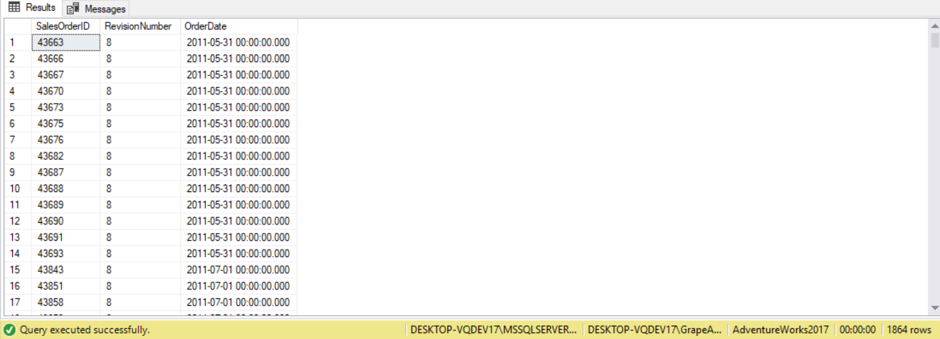
(Include flow chart to explain the different kinds of subqueries)

Subqueries in SQL

SQL supports the ability to write queries inside another query, also known as nested queries. The outermost query is called the outer query and the inner query that is used by the outer query is called the subquery. The result set of a subquery is used by the outer query, and the result set of the outer query is returned to the caller. Subqueries can be used in the SELECT, FROM, WHERE, or HAVING clauses.

There are two different ways to describe subqueries. The first way is based on the result set that is returned: scalar subqueries, multi-valued subqueries, or table-valued subqueries.  A scalar subquery can appear anywhere a scalar expression is expected, meaning it can only return a single value. A multi-value subquery can return multiple values and it can return anywhere multiple values can be expected (most commonly with the WHERE= or WHERE…IN clauses that is providing a list of values). The scalar subquery is typically going to run once for the entire query, meaning it is going to perform better than a correlated subquery.  In addition to scalar and multi-valued result sets, we also have table-valued subqueries, which returns whole a derived table result. which is a table expression.

The second way to describe subqueries is based on their dependency with the outer query. There two different kinds of dependencies: the self-contained model and the correlated subquery model. Self-contained means the subquery has no dependency on table from the outer query. A correlated subquery is dependent on the outer query. The correlated subquery is correlated with the outer query, meaning there’s going to be some type of parameter that we’re passing in from the outer query to the inner query, and in order to run that correlated subquery we must run both together. Typically, correlated subqueries are not going to perform as well, since correlated subqueries are run on a row-by-row basis. Records from the outer query are passed in one row at a time, so performance is not typically good. For performance tuning, always think of each of the queries as sets. See if there’s any way to modify the outer query as to only pass only a distinct list into the inner query, rather than passing all the rows from the outer query.

We can nest subqueries up to 32 levels deep on SQL server. That’s typically far too many levels deep than we need.

Both self-contained and correlated subqueries can return a scalar or multivalued result set.

(Include syntax diagram for subqueries)

Self-contained scalar subqueries

All subqueries have an outer query within which it resides. Self-contained subqueries are independent of the tables in the outer query. They are easy to debug, because we can execute it by itself independently of the outer query to ensure it is working properly. Logically the subquery code is evaluated before the outer query, since the outer query uses the result of the subquery.

Scalar subqueries appear anywhere in the outer query where a single-valued expression can appear (such as WHERE or SELECT). They are used in conjunction with comparison operators (=, !=, <, <= , >, >=) or an expression.

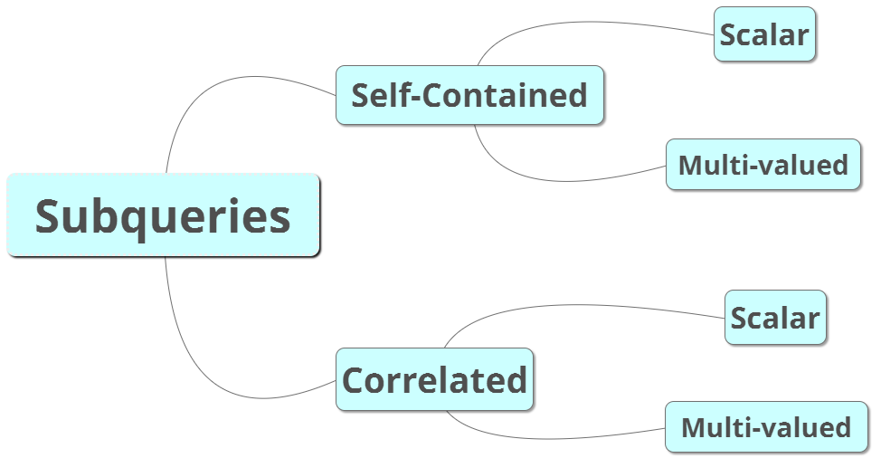
As an example, suppose we’re querying the Sales.SalesOrderHeader table with the following requirements:

• Return all records what have a OrderDate equal to “2013-12-01 00:00:00.000”
• Order the returned records by SalesOrderID
• Number each row returned where the oldest order has a RowNumber of 1, next oldest has a RowNumber of 2, etc
• The result set needs a column named TotalOrders which needs to be populated with the number of total orders that have a OrderDate that is equal to “2013-12-01 00:00:00.000”

The query would go as follows:

USE AdventureWorks2017;
SELECT ROW_NUMBER() OVER(ORDER BY SalesOrderID) AS RowNumber, 
(
    SELECT COUNT(*)
    FROM Sales.SalesOrderHeader
    WHERE ModifiedDate = '2013-12-01 00:00:00.000'
) AS TotalOrders, 
       *
FROM Sales.SalesOrderHeader
WHERE OrderDate = '2013-12-01 00:00:00.000';

 By having this subquery in the column list, this query is able to count the number of SalesOrderHeader rows that have an OrderDate of “2013-12-01 00:00:00.000” and return that information along with the detailed row information about Sales.SalesOrderHeader records having the same OrderDate value.

Subqueries in a SELECT clause as a column expression

If a subquery in the WHERE clause acts as a filter, and a subquery in the FROM clause acts as a derived table, then a subquery in the SELECT clause acts like a column that is to be shown in our output. When a subquery is placed as part of the SELECT list it is used to returned single values. To use a subquery in our SELECT clause, we add it in the place of a column. Typically, subqueries are used in a SELECT clause when we have an aggregate function and no GROUP BY clause. The following query is an example:

(Include code, explanation, and result Database Star)

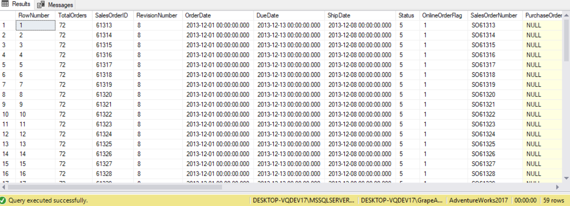
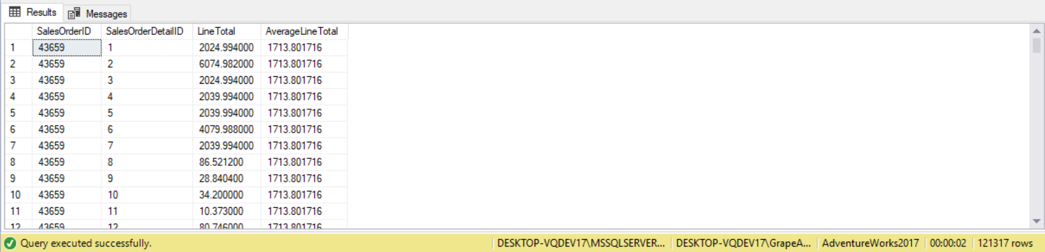
In general, a subquery in a SELECT statement is run only once for the entire query, and its result reused. This is because, the query result does not vary for each row returned. For example, the following displays the LineTotal values and how much they vary from the average:

SELECT SalesOrderID, 
       LineTotal, 
(
    SELECT AVG(LineTotal)
    FROM Sales.SalesOrderDetail
) AS AverageLineTotal
FROM Sales.SalesOrderDetail;

 It is certainly possible to nest a subquery inside another subquery in SQL. In fact, the maximum number of subqueries inside other subqueries we can use is 255. however, we shouldn’t even get close to that many subqueries. However, if we’ve got more than about 5 subqueries then we should look to redesign our query. Let’s say we wanted to see each employee’s salary and the percentage of that salary compared to the average. We can accomplish this using the following query:

(Include code, explanation, and result Database Star)

Subqueries in a WHERE clause as a filter criterion

One place where we can use subqueries is in the WHERE clause. For example, we can use a subquery return all products whose ListPrice is greater than the average ListPrice for all products. To find these records, we need to do two things: first calculate the average price and then use this to compare against each product’s price. Using the subquery will let us do this in one step, as follows:

SELECT ProductID, 
       Name, 
       ListPrice
FROM Production.Product
WHERE ListPrice >
(
    SELECT AVG(ListPrice)
    FROM Production.Product
);

 The subquery eliminated the need for us to find the average ListPrice and then plug it into our query. It means our query automatically adjusts itself to changing data and new averages. The average value is calculated on-the-fly; there is no need for us to “update” the average value within the query.

(Include code, explanation, and results from Pragmatic Works)

What if we have customers with multiple orders on the last OrderDate? In this case, we need a tie-breaker. In the following query, the SalesOrderID is the tie-breaker, bring us the most recent order by OrderDate and SalesOrderID:

Here is the result set:

Using a subquery in a WHERE clause means that we want to use the results of a query as a WHERE clause for another query. If a scalar subquery returns more than one value, the code will fail and return an error message.

The following query runs successfully:

(Include code, explanation, and result from page 159)

Suppose we wish to display all employees that had an above average salary. To find these records, we would need to do two things: find the average salary of all employees and list all employees whose salary is larger than the average:

If the scalar subquery returns no value, the empty result is converted to a NULL. Comparison with a NULL evaluates to UNKNOWN, and the query filter does not return a row. For example, the Employees table has no last name starting with the letter A, so we get returned an empty set in the following query:

(Include code, explanation, and result from page 160)

EXISTS and NOT EXISTS

The EXISTS predicate in T-SQL accepts a subquery as input and returns TRUE if the subquery returns any rows, and FALSE if it doesn’t. The EXISTS predicate allows us to return a row if a given condition exists.

The outer query filters for customers in the Customers table for whom the EXISTS predicate evaluates to TRUE.

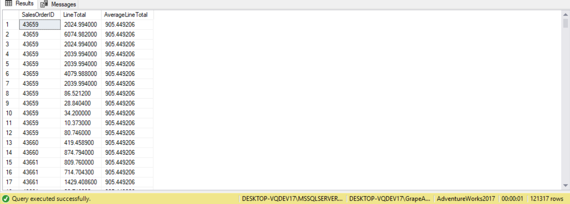
Suppose we need to return all sales orders written by sales people with sales year to date greater than three million dollars.  To do so we can use the EXISTS clause as shown in this example:

SELECT SalesOrderID, 
       RevisionNumber, 
       OrderDate
FROM Sales.SalesOrderHeader
WHERE EXISTS
(
    SELECT 1
    FROM sales.SalesPerson
    WHERE SalesYTD > 3000000
          AND SalesOrderHeader.SalesPersonID = Sales.SalesPerson.BusinessEntityID
);

 As with other predicates, the NOT operator can be used to negate the EXISTS predicate. For example, the following query returns customers from Spain who did not place orders:

(Include code, explanation, and result from page 167)

The EXISTS predicate is optimized for performance, in that the database knows it’s enough to determine whether the subquery returns at least one row or none, and there’s no need to process all qualifying rows. By using an EXISTS predicate, SQL server has to do less work compared to when using a COUNT (*)> 0 predicate. Once one row has been found to satisfy the EXISTS predicate, there’s no need to search any further. The EXISTS version of the query is less resource-intensive than the COUNT(*) version. Failure to use EXISTS instead of COUNT(*) >0 on real-world databases (having tens of thousands to millions rows of data) could take hours to process the query. This concept is similar to the IN predicate.

While the use of star (*) is not good practice, we have an exception with EXISTS. The predicate cares only about the existence of matching rows regardless of what we have in the SELECT list. There may be some minor costs associated with the resolution process, where SQL Server expands the * against metadata info to check we have permissions to query all columns.

Unlike most predicates in T-SQL, the EXISTS predicate uses two-valued logic instead of three-valued logic. This is obviously because there’s no situation where it’s unknown whether a query returns any rows.

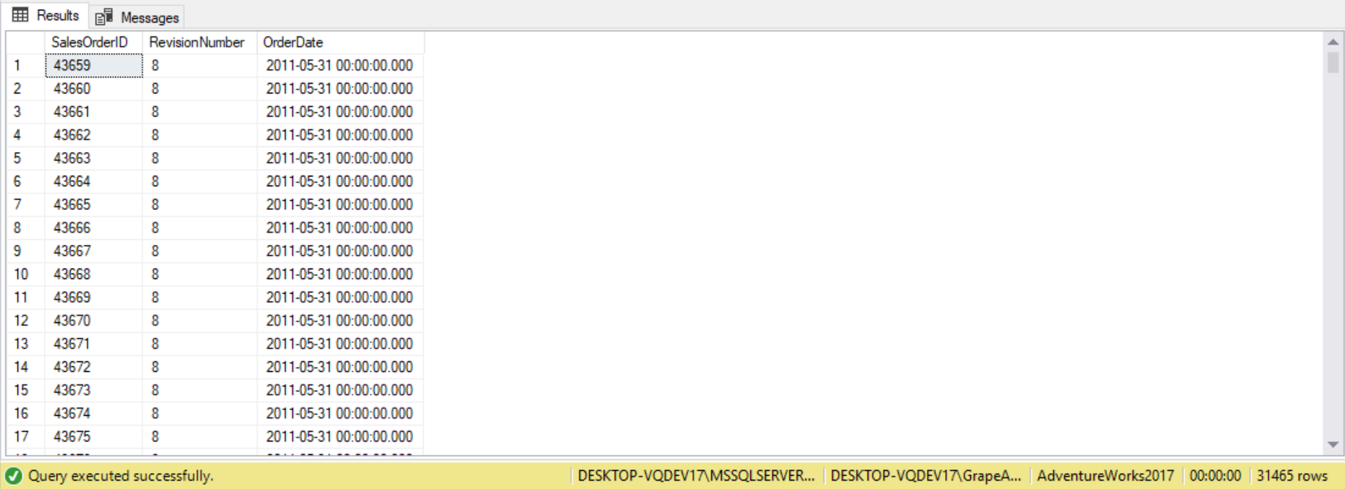
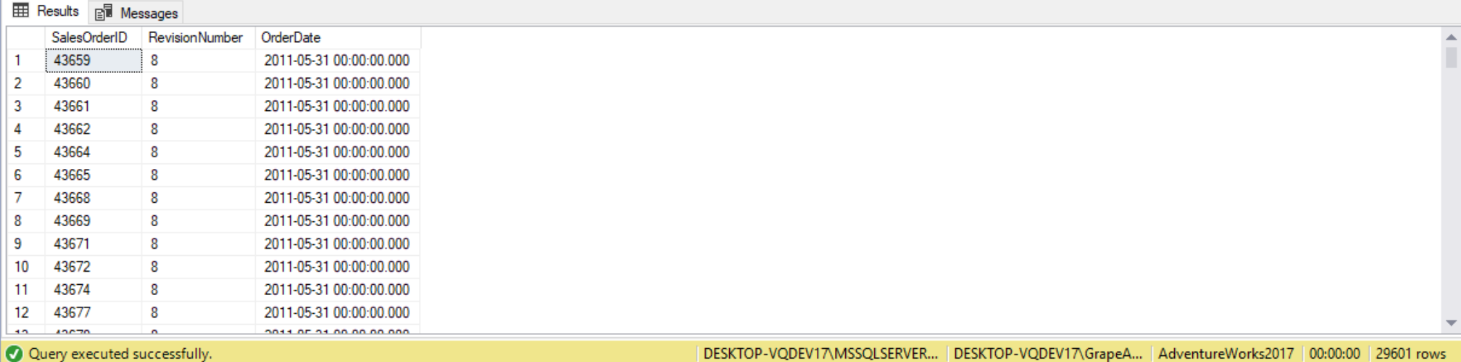
If our subquery returns a NULL value, the EXISTS statement resolves to TRUE. This behavior is unique to the EXISTS clause. In the following example all the SalesOrderHeader rows are returned as the WHERE clause essentially resolved to TRUE:

--This query returns all 31465 records from the Sales.SaleOrderHeader table
SELECT SalesOrderID, 
       RevisionNumber, 
       OrderDate
FROM Sales.SalesOrderHeader
WHERE EXISTS
(
    SELECT NULL
);

 Similar to the NOT IN predicate, the NOT EXIST predicate can be used to return rows that do not match the query. This can be useful for tasks such as handling data feeds:  Sometimes we are tasked with updating or inserting depending on where data in the existing table already exists. Using the NOT EXISTS predicate, we can insert new row while not violating referential integrity. For example, let’s imagine we have a feed of car license-plate numbers and the owner names. We want to update the owner if the car exists, and add the car license-plate and owner if it doesn’t exist. Here we can use the at least one UPDATE and one INSERT statement, and the INSERT statement adds only the new cars. Here’s how we would run such a query:

(Include code, explanation, and result from Subqueries Primer)

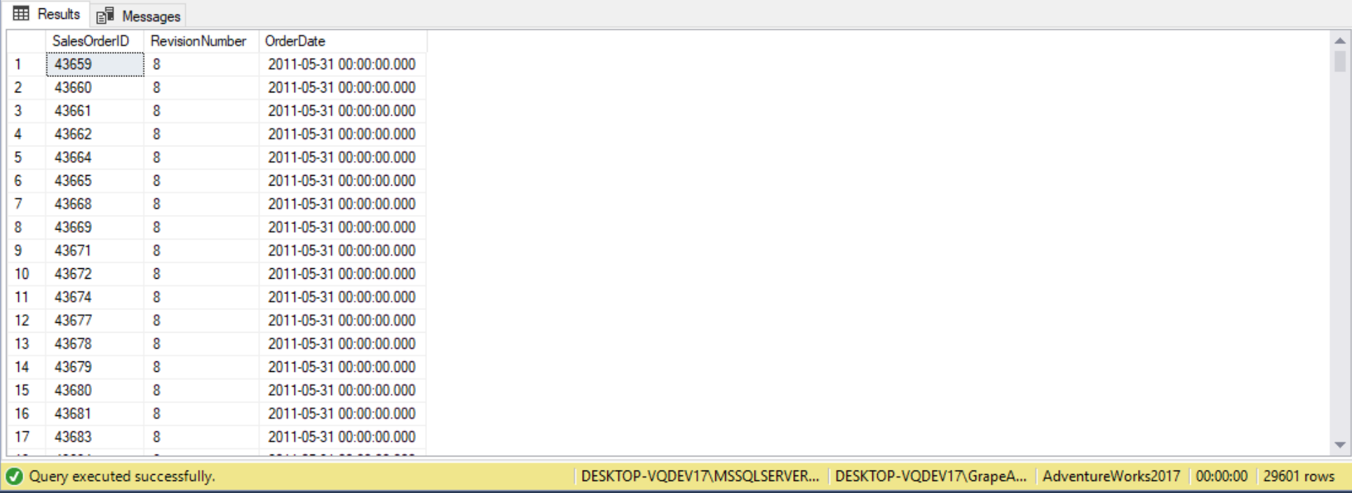
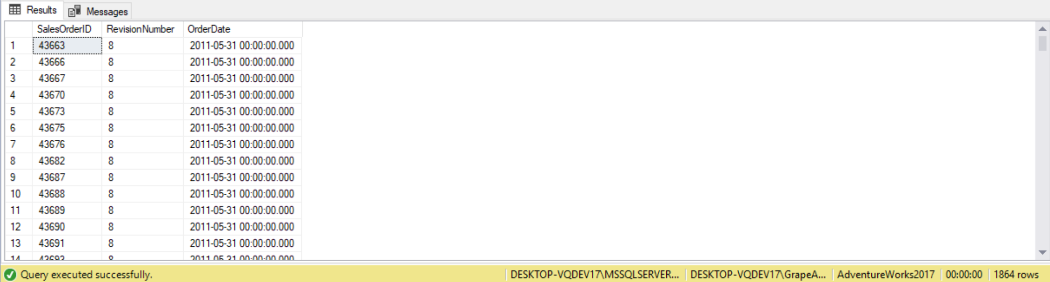
As another example, suppose we want to find all sales orders that were written by salespeople that didn’t have 3,000,000 in year-to-date sales. We can use the following query to accomplish this:

SELECT SalesOrderID, 
       RevisionNumber, 
       OrderDate
FROM Sales.SalesOrderHeader
WHERE SalesPersonID NOT IN
(
    SELECT SalesPerson.BusinessEntityID
    FROM sales.SalesPerson
    WHERE SalesYTD > 3000000
          AND SalesOrderHeader.SalesPersonID = Sales.SalesPerson.BusinessEntityID
);

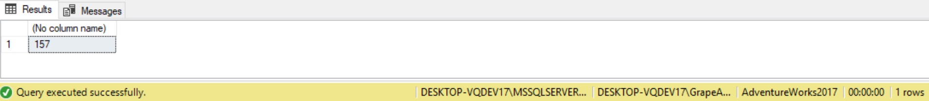
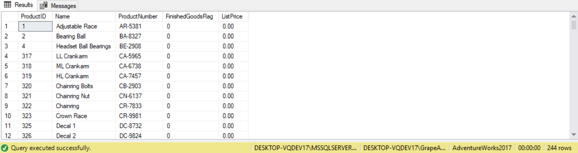
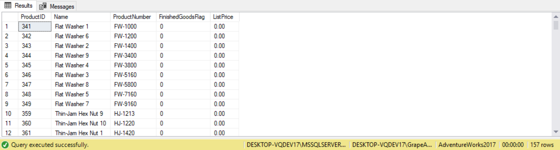
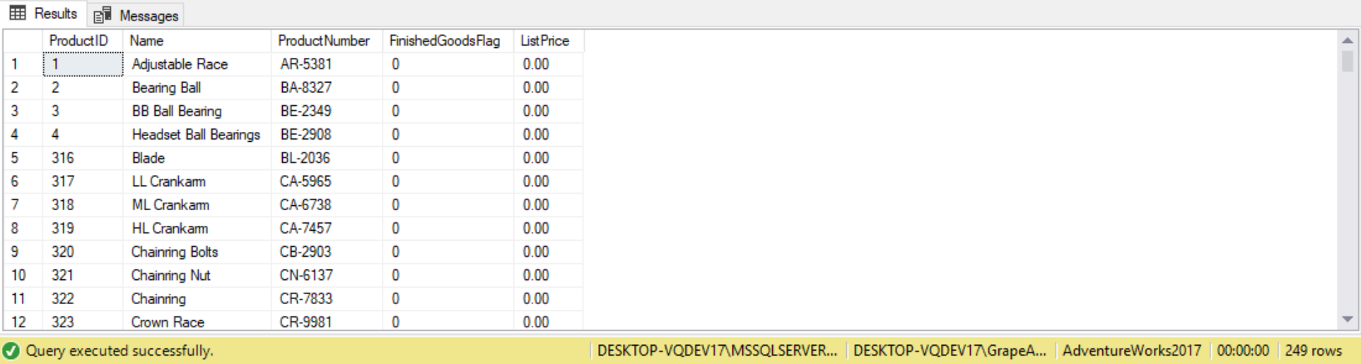
 As a final demo for this section, we use both the EXISTS and NOT EXISTS predicates to query the Production.BillofMaterials table. The queries will return the following:

1. Count of products not listed in BillOfMaterials
2. ProductIDs, including Names and ProductNumbers, that have no subcomponents
3. Product IDs, including Names and ProductNumbers, that aren’t in a subcomponent
4. Product IDs, including Names and ProductNumbers, that are a subcomponent

The following are the queries and results for that return each respective requirements listed above:

SELECT COUNT(1)
FROM Production.Product P
WHERE P.SellEndDate IS NULL
      AND p.DiscontinuedDate IS NULL
      AND NOT EXISTS
(
    SELECT 1
    FROM Production.BillOfMaterials BOM
    WHERE BOM.ProductAssemblyID = p.ProductID
          OR BOM.ComponentID = p.ProductID
);

SELECT P.ProductID, 
       P.Name, 
       P.ProductNumber, 
       P.FinishedGoodsFlag, 
       P.ListPrice
FROM Production.Product P
WHERE P.SellEndDate IS NULL
      AND p.DiscontinuedDate IS NULL
      AND NOT EXISTS
(
    SELECT 1
    FROM Production.BillOfMaterials BOM
    WHERE P.ProductID = BOM.ProductAssemblyID
);

SELECT P.ProductID, 
       P.Name, 
       P.ProductNumber, 
       P.FinishedGoodsFlag, 
       P.ListPrice
FROM Production.Product P
WHERE P.SellEndDate IS NULL
      AND p.DiscontinuedDate IS NULL
      AND NOT EXISTS
(
    SELECT 1
    FROM Production.BillOfMaterials BOM
    WHERE P.ProductID = BOM.ComponentID
);

SELECT P.ProductID, 
       P.Name, 
       P.ProductNumber, 
       P.FinishedGoodsFlag, 
       P.ListPrice
FROM Production.Product P
WHERE P.SellEndDate IS NULL
      AND p.DiscontinuedDate IS NULL
      AND EXISTS
(
    SELECT 1
    FROM Production.BillOfMaterials BOM
    WHERE P.ProductID = BOM.ComponentID
);

Subqueries in the HAVING clause as a table specification

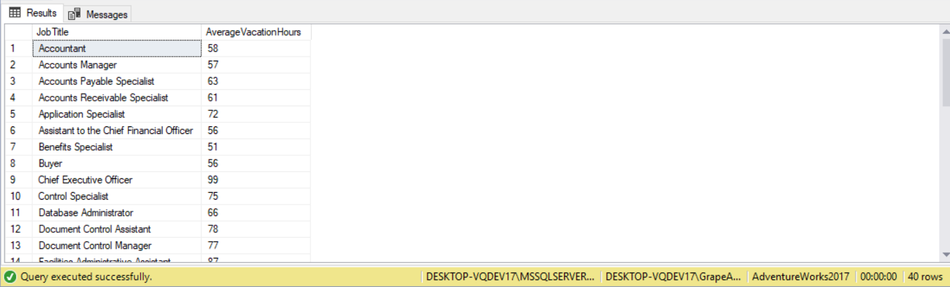
HAVING is the equivalent of the WHERE clause but only in GROUP BY situations or the result of an aggregate function. For example, it is now possible to compare the average of a group to the overall average. In this demo we’re selecting employee job titles having remaining vacation hours greater than the overall average for all employees. The following is how the query would go:

SELECT JobTitle, 
       AVG(VacationHours) AS AverageVacationHours
FROM HumanResources.Employee
GROUP BY JobTitle
HAVING AVG(VacationHours) >
(
    SELECT AVG(VacationHours)
    FROM HumanResources.Employee
);

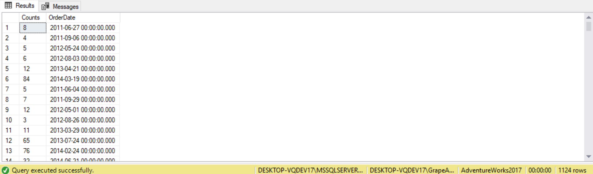
 Suppose we want to produce a result set that contains the Sales.SalesOrderHeader.OrderDate and the number of orders for each date, where the number of orders exceeds the number of orders taken on ’2006-05-01’. This is can be accomplished using a subquery in the HAVING clause, like follows:

SELECT COUNT(*) AS Counts, 
       OrderDate
FROM Sales.SalesOrderHeader
GROUP BY OrderDate
HAVING COUNT(*) >
(
    SELECT COUNT(*)
    FROM Sales.SalesOrderHeader
    WHERE OrderDate = '2006-05-01 00:00:00.000'
);

 Subquery in a Function call

Subqueries can also be used in a function call. Suppose we want to display the number of days between the OrderDate and the maximum OrderDate for each Sales.SalesOrderHeader records. The query would go as follows:

SELECT SalesOrderID, 
       OrderDate, 
       DATEDIFF(dd, OrderDate,
(
    SELECT MAX(OrderDate)
    FROM Sales.SalesOrderHeader
)) AS DaysBetweenOrders, 
(
    SELECT MAX(OrderDate)
    FROM Sales.SalesOrderHeader
) AS MaxOrderDate
FROM Sales.SalesOrderHeader;

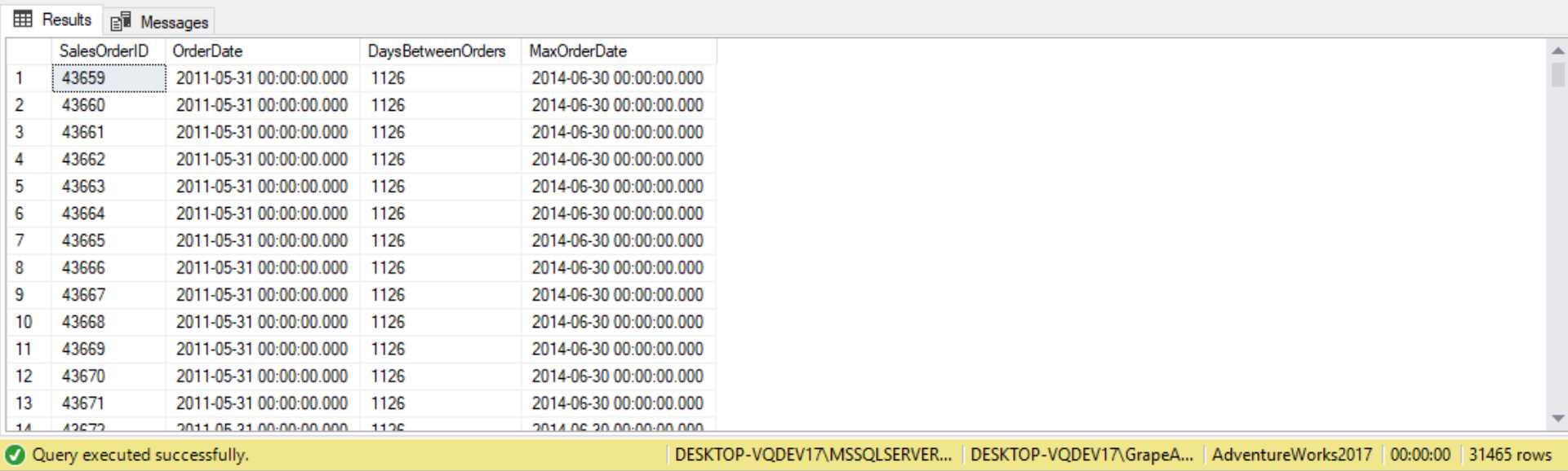
 Here, both subqueries return the max OrderDate in the Sales.SalesOrderHeader table. But the first subquery is used to pass a date to the second parameter of the DATEDIFF function.

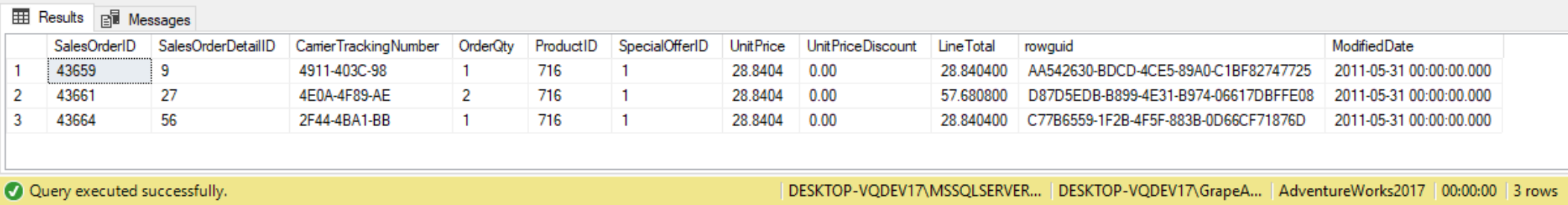
Subquery to control the TOP clause

We can also use a subquery to control a TOP clause. For example, the following code uses the OrderQty value returned from the subquery to identity the value that will be used in the TOP clause. By using a subquery to control the number of rows that TOP clause returns, allows us to build a subquery that will dynamically identify the number of rows returned from your query at runtime:

SELECT TOP (SELECT TOP 1 OrderQty
            FROM Sales.SalesOrderDetail
            ORDER BY ModifiedDate) *
FROM Sales.SalesOrderDetail
WHERE ProductID = 716;

 Self-contained multivalued subquery

Multivalued subquery returns multiple values as a single column. We can use predicates such as the IN predicate to operate on a multivalued subquery. Other predicates that work on multivalued subqueries include: SOME, ANY, and ALL.

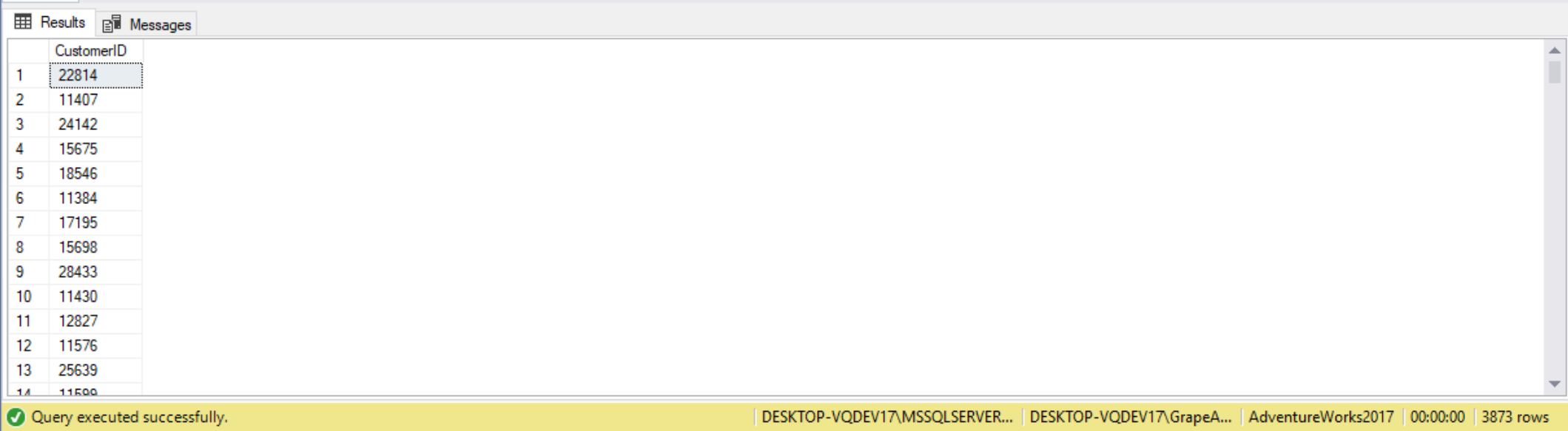
As another example, here we use a subquery to list all customers whose territories have sales below $5,000,000.

SELECT DISTINCT 
       CustomerID
FROM Sales.SalesOrderHeader
WHERE TerritoryID IN
(
    SELECT TerritoryID
    FROM Sales.SalesTerritory
    WHERE SalesYTD < 5000000
);

 Another example here demonstrates using multiple self-contained subqueries, both single-valued and multivalued, in the same subquery.

(Include a better code, explanation, and result than from page 163)

IN AND NOT IN

The IN operator allows us to conduct multiple match tests compactly in one statement. In its simplest form the IN statement matches a column to a list of values. TRUE is returned if there is a match to any of the values returned by the subquery.  A main advantage of using subqueries with the IN operator, is the list’s contents are the subquery results, making the query dynamic and flexible. For example, query to returns sales people with sales year to date greater than three million dollars:

SELECT SalesOrderID, 
       OrderDate, 
       AccountNumber, 
       CustomerID, 
       SalesPersonID, 
       TotalDue
FROM Sales.SalesOrderHeader
WHERE SalesPersonID IN
(
    SELECT BusinessEntityID
    FROM Sales.SalesPerson
    WHERE Bonus > 5000
);

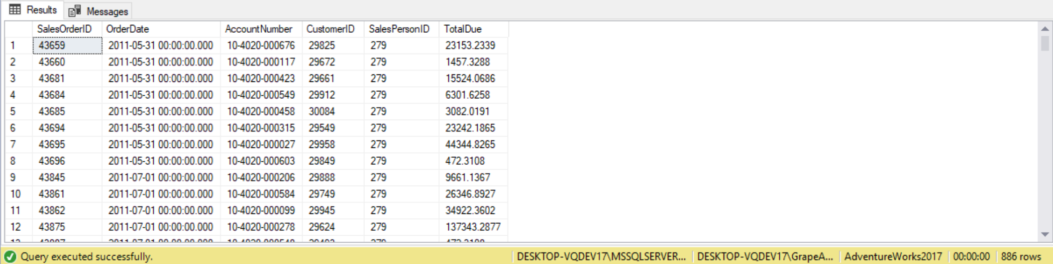
 Because we used the IN predicate, our query is valid with any number of values returned- none, one, or more. Using IN is a more elegant substitute to using a bunch of OR predicates.

The advantage here is that as sales persons sell more or less, the list of sales person ID’s returned adjusts.

When the comparison list contains NULL, any value compared to that list returns false. For instance, the following query returns zero rows. This is because the IN clause always returns false. This is in contrast to EXIST, which returns TRUE even when the subquery returns NULL.

Just like with any other predicates, the IN predicate can be negated with the NOT operator. For example, the following query returns customers who did not place any orders:

(Include code, explanation, and result from page 161)

It is good practice to qualify subqueries to exclude NULLs.

The subquery returns all customer ids from the Orders table, in other words all customer ids that have made an order. The outer query returns customer ids from the Customers table that are not in the result set returned by the subquery, in other words only customer ids that haven’t made any order. The database engine is smart enough to consider removing duplicates without us asking to do so explicitly using the DISTINCT clause.

Self-contained table-valued subquery

Subquery in the FROM clause as a table specification

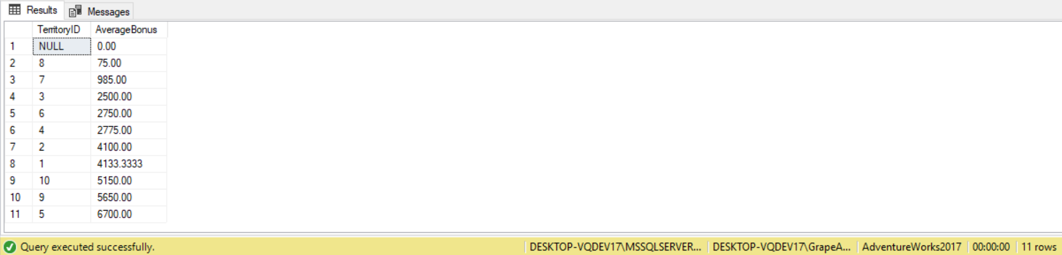
Another place we can use a subquery is in a FROM clause. When subqueries are used in the FROM clause they act as a table that you can use to select columns and join to other tables. These tables are known as derived tables. The following query is an example, where we select territories and their average bonuses:

SELECT TerritoryID, 
       AverageBonus
FROM
(
    SELECT TerritoryID, 
           AVG(Bonus) AS AverageBonus
    FROM Sales.SalesPerson
    GROUP BY TerritoryID
) AS TerritorySummary
ORDER BY AverageBonus;

 When this query run, the subquery is first run and the results created.  The results are then used in the FROM clause as if it were a table.  When used by themselves these types of queries aren’t very fascinating; however, when used in combination with other tables they are. For instance, we can use the results of this subquery to join to other tables, like follows:

SELECT SP.TerritoryID, 
       SP.BusinessEntityID, 
       SP.Bonus, 
       TerritorySummary.AverageBonus
FROM
(
    SELECT TerritoryID, 
           AVG(Bonus) AS AverageBonus
    FROM Sales.SalesPerson
    GROUP BY TerritoryID
) AS TerritorySummary
INNER JOIN Sales.SalesPerson AS SP ON SP.TerritoryID = TerritorySummary.TerritoryID;

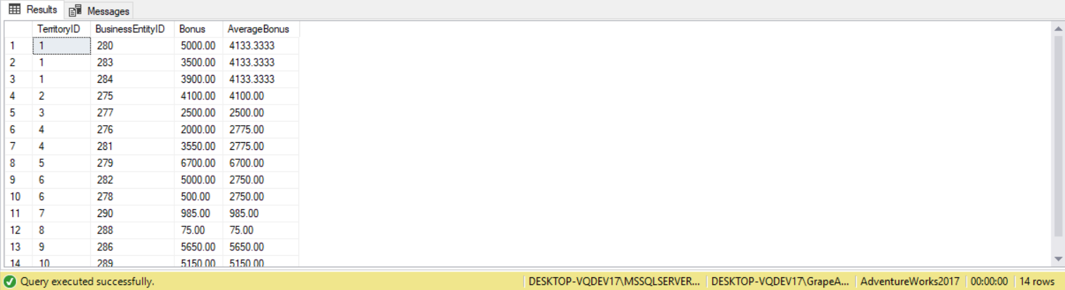
A derived table must be aliased so that we can reference the results. First, we’re selecting columns from two tables: the SP and TerritorySummay tables. The TerritorySummary table is actually the result of the subquery, which is the TerritoryID and AverageBonus columns. We’re then joining that subquery to the SP table. By using derived tables we are able to summarize using one set of fields and report on another.  In this case we’re summarizing by TerritoryID but report by each sales person (BusinessEntityID). We may think we could simple replicate this query using an INNER JOIN , but we can’t as the final GROUP BY for the query would have to include BusinessEntityID, which would then throw-off the Average calculation.

Derived Tables and Aggregate Functions

When working with aggregate functionswe may have wanted to first summarize some values and then get the overall average.  For instance, suppose we want to know the average bonus given for all territories. If we run the following query we will get an error message:

SELECT AVG(SUM(Bonus))
FROM Sales.SalesPerson
GROUP BY Bonus;

 To get the average bonus for territories we first have to calculate the total bonus by territory, and then take the average. Once way to do this is with derived tables.  In the following query the derived table is used to summarize sales by territory.  These are then fed into the AVG() function to obtain an overall average.

SELECT AVG(B.TotalBonus)
FROM
(
    SELECT TerritoryID, 
           SUM(Bonus) AS TotalBonus
    FROM Sales.SalesPerson
    GROUP BY TerritoryID
) AS B;

 Joining Derived Tables with a real table

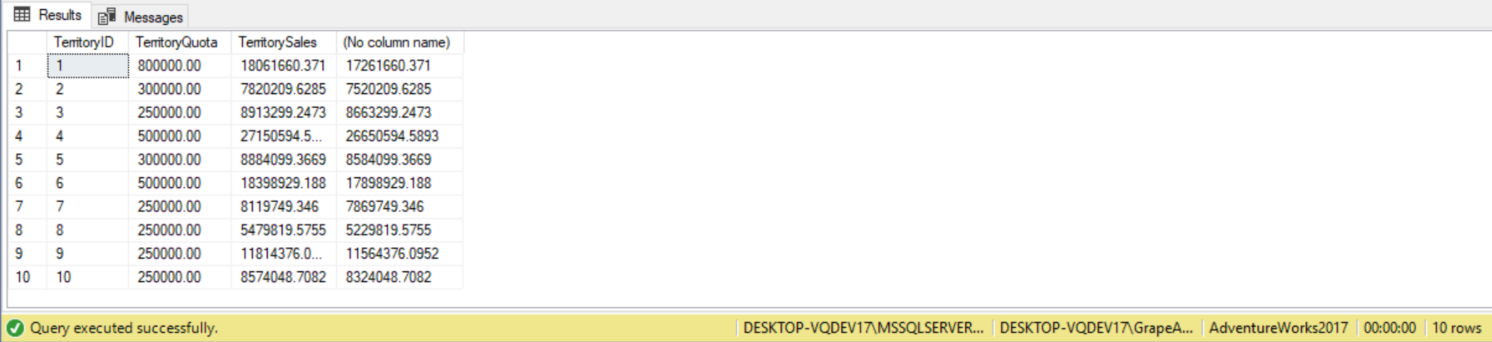
We can also join two derived tables together!  This can come in handy when we need to aggregate data from two separate tables and combine them together.  In the following demo we’re going to do a comparison of TerritorySales to TerritoryQuota.  We’ll do this by summing sales figures and quotas by Territory. Here are the two SELECT statements we’ll use to summarize the sales figures:

--First SELECT Statement
SELECT TerritoryID, 
       SUM(SalesQuota) AS TerritoryQuota
FROM Sales.SalesPerson
GROUP BY TerritoryID;

--Second SELECT Statement
SELECT SOH.TerritoryID, 
       SUM(SOH.TotalDue) AS TerritorySales
FROM Sales.SalesOrderHeader AS SOH
GROUP BY SOH.TerritoryID;

To obtain the comparison we’ll match these two results together by territory ID, using the FROM clause:

SELECT Quota.TerritoryID, 
       Quota.TerritoryQuota, 
       Sales.TerritorySales, 
       Sales.TerritorySales - Quota.TerritoryQuota
FROM
(
    SELECT TerritoryID, 
           SUM(SalesQuota) AS TerritoryQuota
    FROM Sales.SalesPerson
    GROUP BY TerritoryID
) AS Quota
INNER JOIN
(
    SELECT SOH.TerritoryID, 
           SUM(SOH.TotalDue) AS TerritorySales
    FROM Sales.SalesOrderHeader AS SOH
    GROUP BY SOH.TerritoryID
) AS Sales ON Quota.TerritoryID = Sales.TerritoryID;

 In many cases what we can do with derived tables we can do with joins; however, there are special cases where this isn’t the case.  The best example where a derived tables shines is when we need to use two aggregate functions, such as taking the average of a sum. It is best to go with the simplest and easiest solution (which typically is an INNER JOIN, but not every solution is solved as such).

Correlated subqueries

A correlated subquery is when a subquery refers to a column that exists in the outer query. The subquery and the outer query are said to be correlated, as they are linked to each other. This means that correlated subqueries cannot be executed independently of the outer query. In correlated subqueries, the inner SELECT query is dependent on the values of the outer SELECT.

Logically, the subquery is evaluated separately for each outer row. For example, the following query returns orders with the maximum order ID for each customer:

(Include code, explanation, and result from page 164)

The outer query filters orders where the order id is equal to the value returned by the subquery. An outer table instance of Orders o1 is correlated to an inner instance of Orders o2 where the inner customer id o2.custid is equal to the outer customer id o1.custid, and the subquery returns the maximum ordered id for from those filtered orders. So, for each row in o1 we get returned the by the subquery the maximum order id for the current customer. If the order ids between the outer query and subquery match, the query returns the outer row.

(Include code, explanation, and result from Subqueries Primer)

A correlated subquery can just as easily appear using the SELECT clause. For instance, the following query returns the SalesOrderDetail, LineTotal, and AverageLineTotal for the overall sales order. The average we’re calculating varies for each sales order. We can use the value from the outer query and incorporate into the filter criteria of the subquery. The outer query is used to retrieve all SalesOrderDetail lines.  The subquery is used to find and summarize sales order details lines for a specific SalesOrderID.

SELECT SalesOrderID, 
       SalesOrderDetailID, 
       LineTotal, 
(
    SELECT AVG(LineTotal)
    FROM Sales.SalesOrderDetail
    WHERE SalesOrderID = SOD.SalesOrderID
) AS AverageLineTotal
FROM Sales.SalesOrderDetail SOD;

 Since a correlated subquery is dependent on the outer query, they are harder to debug than self-contained subqueries. With correlated subqueries it is more difficult to debug and figure out why something is not working, or why the proper results are not getting returned.

Suppose we’re querying the Sales.OrderValues view to return for each order the percentage of the current order value out of the customer total. We write an outer query against one instance of the OrderValues view called o1. In the SELECT list, we divide the current value by the result of a correlated subquery against a second instance of OrderValues called o2, which returns the current customer’s total. Here’s how the query would go:

(Include code, explanation, and result from page 166)

The CAST function is used to convert the datatype of the expression to NUMERIC with a precision (number of digits total) of 5 and a scale of 2 (number of decimal points).

Correlated Subqueries in WHERE clause

Just like with other queries we can create a correlated sub query to be used with the IN clause.  For example, the following query uses the IN clause to return all sales orders written by sales people with sales year to date greater than three million dollars:

SELECT SalesOrderID, 
       RevisionNumber, 
       OrderDate
FROM Sales.SalesOrderHeader
WHERE SalesPersonID IN
(
    SELECT SalesPerson.BusinessEntityID
    FROM sales.SalesPerson
    WHERE SalesYTD > 3000000
          AND SalesOrderHeader.SalesPersonID = Sales.SalesPerson.BusinessEntityID
);

 

As IN returns TRUE if the tested value is found in the comparison list, NOT IN returns TRUE if the tested value is not found.  Taking the same query from above, we can find all Sales orders that were written by sales people that didn’t write 3,000,000 in year-to-date sales using the following query:

SELECT SalesOrderID, 
       RevisionNumber, 
       OrderDate
FROM Sales.SalesOrderHeader
WHERE SalesPersonID NOT IN
(
    SELECT SalesPerson.BusinessEntityID
    FROM sales.SalesPerson
    WHERE SalesYTD > 3000000
          AND SalesOrderHeader.SalesPersonID = Sales.SalesPerson.BusinessEntityID
);

 When the comparison list only contains the NULL value, then any value compared to that list returns false. For instance, the following query returns zero rows.  This is because the IN clause always returns false. Contrast this to EXISTS, which returns TRUE even when the subquery returns NULL.

SELECT SalesOrderID, 
       RevisionNumber, 
       OrderDate
FROM Sales.SalesOrderHeader
WHERE SalesOrderID IN
(
    SELECT NULL
);

 Correlated Subqueries in HAVING clause

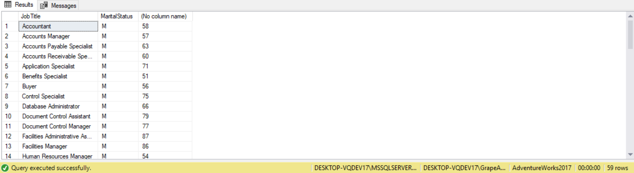
As with any other subquery, subqueries in the HAVING clause can be correlated with fields from the outer query. Suppose we further group the job titles by marital status and only want to keep those combinations of job titles and martial statuses whose vacation hours are greater than those for their corresponding overall marital status.  In other words, we want to answer questions similar to “do married accountants have, on average, more remaining vacation, than married employees in general?” One way to find out is to us the following query:

SELECT JobTitle, 
       MaritalStatus, 
       AVG(VacationHours)
FROM HumanResources.Employee AS E
GROUP BY JobTitle, 
         MaritalStatus
HAVING AVG(VacationHours) >
(
    SELECT AVG(VacationHours)
    FROM HumanResources.Employee
    WHERE HumanResources.Employee.MaritalStatus = E.MaritalStatus
);

 With a correlated query, only fields used in the GROUP BY can be used in the inner query.  For instance, out of curiosity, we tried replacing MaritalStatus with Gender and got an error.

SELECT JobTitle, 
       MaritalStatus, 
       AVG(VacationHours)
FROM HumanResources.Employee AS E
GROUP BY JobTitle, 
         MaritalStatus
HAVING AVG(VacationHours) >
(
    SELECT AVG(VacationHours)
    FROM HumanResources.Employee
    WHERE HumanResources.Employee.Gender = E.Gender
);

 As another example, suppose we want to calculate rebate amounts for those customer that have purchased more than $150000 worth of products before taxes in the year 2013. We can accomplish this using a correlated subquery in the HAVING clause, as follows:

SELECT soh.CustomerID, 
       SUM(soh.SubTotal) AS TotalPurchase, 
       SUM(soh.SubTotal) * .10 AS Rebate
FROM Sales.SalesOrderHeader AS soh
WHERE YEAR(soh.OrderDate) = '2013'
GROUP BY soh.CustomerID
HAVING
(
    SELECT SUM(soh2.SubTotal)
    FROM Sales.SalesOrderHeader AS soh2
    WHERE soh2.CustomerID = soh.CustomerID
          AND YEAR(soh2.OrderDate) = '2013'
) > 150000
ORDER BY Rebate DESC;

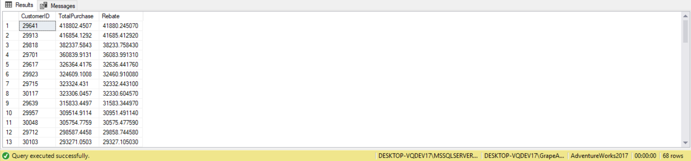
The correlated subquery code in the above query uses the CustomerID from the GROUP BY clause in the outer query within the correlated subquery. The correlated subquery will be executed once for each row returned from the GROUP BY clause. This allows the HAVING clause to calculated the total amount of products sold to each CustomerID from the outer query by summing the values of the SubTotal column on each SalesOrderHeader record where the record is associated with the CustomerID from the outer query. The query only returns a row where the CustomerID in has purchased more than $150,000 worth of product.

Correlated Subquery with a different table

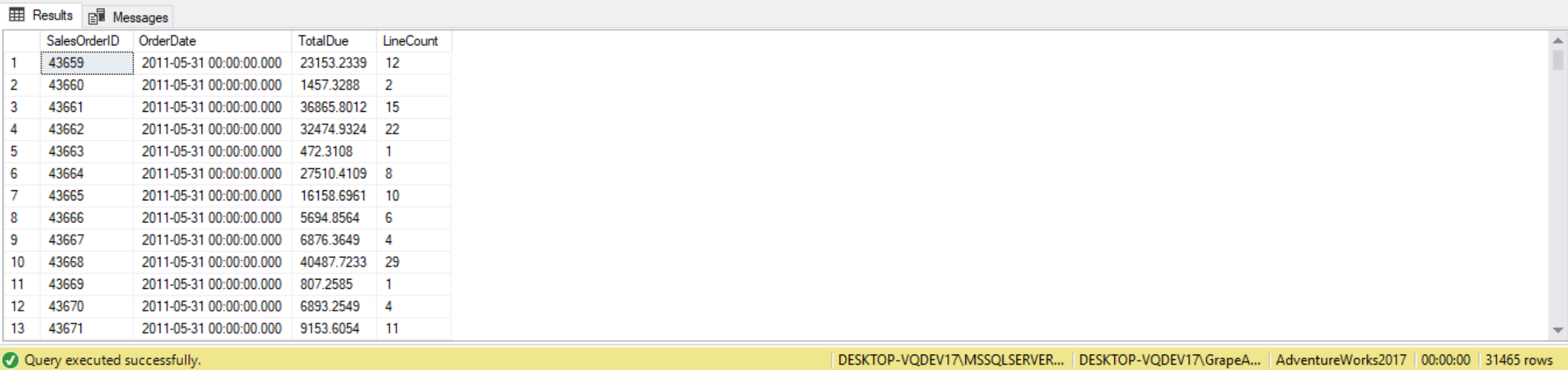
A Correlated subquery, (or any subquery), can use a different table than the outer query.  This can come in handy when we’re working with a “parent” table, such as SalesOrderHeader, and you want to include in result a summary of child rows, such as those from SalesOrderDetail. The following code uses a correlated subquery in our SELECT statement to return the COUNT of SalesOrderDetail lines, in addition to SalesOrderID, OrderDate and TotalDue.  We ensure we are counting the correct SalesOrderDetail item by filtering on the outer query’s SalesOrderID.

SELECT SalesOrderID, 
       OrderDate, 
       TotalDue, 
(
    SELECT COUNT(SalesOrderDetailID)
    FROM Sales.SalesOrderDetail
    WHERE SalesOrderID = SO.SalesOrderID
) AS LineCount
FROM Sales.SalesOrderHeader SO;

 Correlated Subqueries versus Inner Joins

Joins and subqueries are both used to combine data from different tables into a single result. Though both can return the same results, there are advantages and disadvantages to each method.

Joins are used in the FROM clause of the WHERE statement; however, we find subqueries used in most clauses such the SELECT, WHERE, FROM, and HAVING clauses.

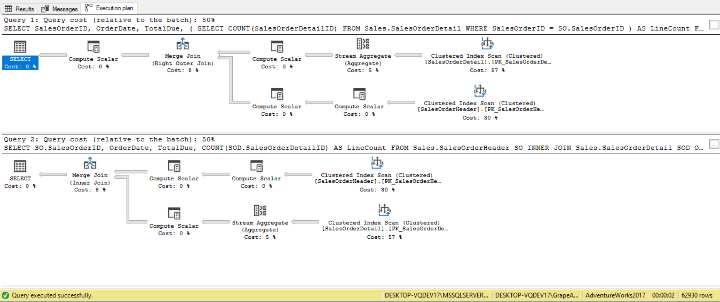
Suppose we’re using the AdventureWorks2017 database to return a detailed listing of all sales orders and the number of order details lines for each order. The following correlated subquery and inner join queries return the same result to accomplish this:

--Subquery Solution: Returns 31465 records
SELECT SalesOrderID, 
       OrderDate, 
       TotalDue, 
(
    SELECT COUNT(SalesOrderDetailID)
    FROM Sales.SalesOrderDetail
    WHERE SalesOrderID = SO.SalesOrderID
) AS LineCount
FROM Sales.SalesOrderHeader SO;

--INNER JOIN Solution: Returns 31465 records
SELECT SO.SalesOrderID, 
       OrderDate, 
       TotalDue, 
       COUNT(SOD.SalesOrderDetailID) AS LineCount
FROM Sales.SalesOrderHeader SO
     INNER JOIN Sales.SalesOrderDetail SOD ON SOD.SalesOrderID = SO.SalesOrderID
GROUP BY SO.SalesOrderID, 
         OrderDate, 
         TotalDue;

Typically, subqueries are slower, since the correlated subquery has to “execute” once for each row returned in the outer query, whereas the INNER JOIN only has to make one pass through the data. In this case, the query plan is the same! Most SQL DBMS optimizers are really good at figuring out the best way to execute your query.  They’ll take our syntax, such as a subquery, or INNER JOIN, and use them to create an actual execution plan. Generally speaking, if there are more direct means to achieve the same result, such as using an inner join, that would be a better option since subqueries can become very inefficient.

(Include more examples with execution plans)

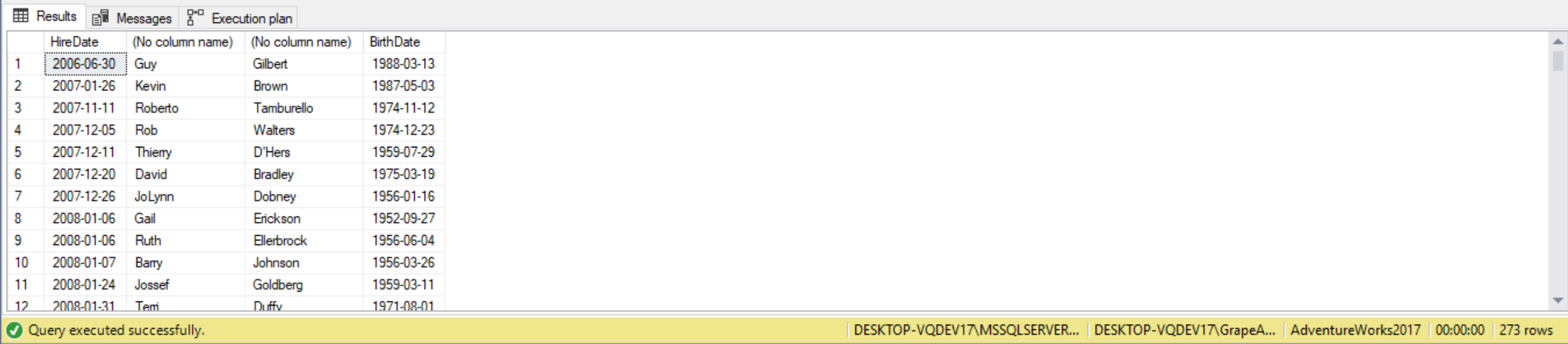
As another example, the following subquery returns employee information. The query combines data from two different table, using subqueries in both the FROM and WHERE clause. Also, each correlated subquery’s WHERE clause is restricting the rows returned to those equal to the Employee.BusinessEntityID.

SELECT E.HireDate, 
(
    SELECT FirstName
    FROM Person.Person P1
    WHERE P1.BusinessEntityID = E.BusinessEntityID
), 
(
    SELECT LastName
    FROM Person.Person P2
    WHERE P2.BusinessEntityID = E.BusinessEntityID
), 
       E.BirthDate
FROM HumanResources.Employee E
WHERE
(
    SELECT PersonType
    FROM Person.Person T
    WHERE T.BusinessEntityID = E.BusinessEntityID
) = 'EM'
ORDER BY HireDate, 
(
    SELECT FirstName
    FROM Person.Person P1
    WHERE P1.BusinessEntityID = E.BusinessEntityID
);

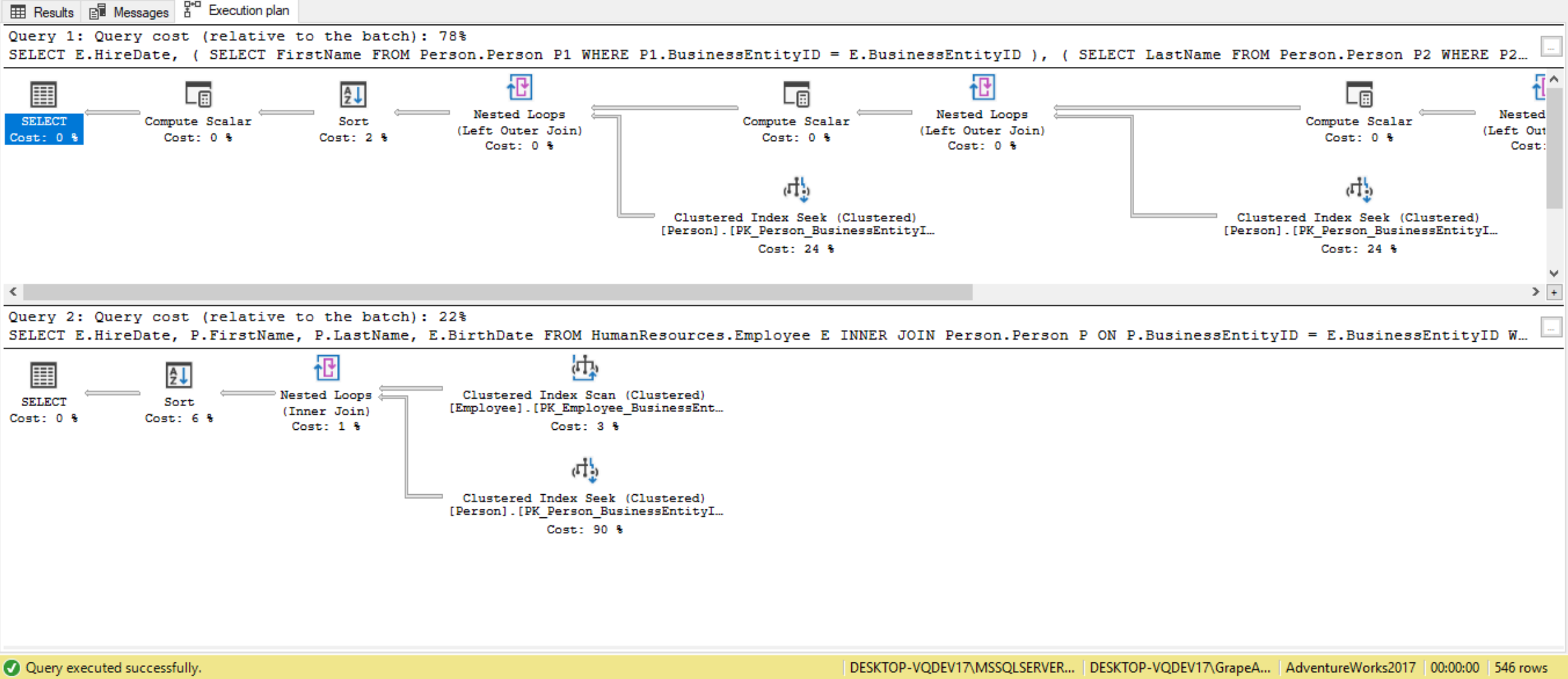
 We can convert the above code that is using subqueries to instead use an inner join, like follows:

SELECT E.HireDate, 
       P.FirstName, 
       P.LastName, 
       E.BirthDate
FROM HumanResources.Employee E
     INNER JOIN Person.Person P ON P.BusinessEntityID = E.BusinessEntityID
WHERE P.PersonType = 'EM'
ORDER BY E.HireDate, 
         P.FirstName;

 Looking at the execution plan we see that in the case of the subquery each subquery results in a nested loop, meaning four nested loops in total. The less nested loop a query uses the better. In the case of the inner join query, we see there is only one nested loop involved. So, after observing both the SQL and query plans for each set of statements you can see that inner join is superior in several ways. In the execution plan below, the top box is the actual execution plan for the subquery method, whereas the bottom box is the actual execution plan for the inner join method:

Performance considerations for correlated subqueries

There are some performance considerations we should be aware of when writing T-SQL statements containing correlated subqueries. The performance isn’t bad when the outer query contains a small number of rows. But when the outer query contains a large number of rows it doesn’t scale well from a performance perspective. This is because the correlated subquery is executed for every row in the outer query. Therefore, when the outer query contains more and more rows a correlated subquery has to be executed many times, and therefore the query will take longer to run. If we find performance of our correlated subquery is not meeting our requirements, then we should look for alternatives solutions, such as queries that use an INNER or OUTER JOIN, or ones that return a smaller number of candidate rows from the outer query.

To summarize, joins excel at combining data from two tables, subqueries are best when testing for the existence of a value from one table found in another.

Beyond the fundamentals of subqueries

Returning previous or next values

Suppose we’re querying the Orders table to return for each order the information about the current order and also the previous order id. This is tricky because rows in a table have no order. One way to achieve this is to look for the maximum value that is smaller than the current value. We use a correlated subquery, like follows:

(Include code, explanation, and result from page 168)

Notice that if there’s no order before the first order, the subquery returns a NULL for the first order. Similarly, we can also get information on the next order id, by querying for the minimum value that is greater than the current value, like in the following query:

(Include code, explanation, and result from page 168)

If there’s no order after the last order, the subquery returns a NULL for the last order.

Note that the previous two queries could also be accomplished using T-SQL window functions called LAG and LEAD.

Using running aggregates

Aggregate calculations that accumulate in value based on some order are called running aggregates. For example, we can use the Sales.OrderTotalsByYear view to calculate the running total quantity up to an including a specified year. We query one instance of the view (o1) to return for each year the current year and quantity. We also use a correlated subquery against the second instance of the view (o2) to calculate the running total quantity. The subquery filters all rows in o2 where the order year is smaller than or equal to the current year in o1, and sum the quantities from o2. Here’s how the query would go:

(Include code, explanation, and result from page 170)

The inner query takes the same sum as the outer query, but it doesn’t use grouping, and it sums all orders with an order date greater or equal to the order date of the outer query. If we run this against tables with many rows, we will get a lot of I/O, which can have a performance impact.

Note that in T-SQL we have window aggregate functions which can be used to calculate running totals more easily and efficiently.

Subqueries, Joins, and Unions in a query

(CONSULT WENZEL)

Creating Histograms

One scenario where derived tables are useful is when we require histograms, which depict the distribution of count of values. Suppose we’re using the AdventureWorks2017 database and we wish to have a histogram showing the number of orders placed by a customer. Once we have the counts, we need to get a “count of counts” which is generated by another GROUP BY clause. If we want a quasi-graphical representation of the histogram, we just have to change COUNT(*) to REPLICATE(‘*’,COUNT(*)), which produces an instant bar chart! The code for this is as follows:

(Use the Advanced BOOK code on AdventureWorks SalesOrderHeader)

Dealing with misbehaving subqueries

NULL trouble

There may be some problems that arise when we forget about NULLs and the three-valued predicate logic when working with subqueries. For example, the following query is supposed to return customers who did not place orders:

(Include code, explanation, and result from page 170)

Currently, the query does seem to work as expected. Let’s run a query that inserts a new order into the Orders table with a NULL customer id:

(Include code, explanation, and result from page 171)

We now run the query again:

(Include code, explanation, and result from page 171 – second one)

This time the query returns an empty return set. The culprit here is the NULL customer id record that we added to the Orders table. The IN predicates returns TRUE for customers who placed orders in the subquery. The NOT operator negates the IN predicate, so those customer records get discarded since they not evaluate to FALSE by the NOT operator. What we expected is that any customer id appearing in the Orders table will not get returned. However if the IN predicate evaluates to UNKNOWN for customer ids in the Customers table (outer table) that do not appear in the customer IDs attributes of the Orders table (subquery table). This is because the IN predicate evaluates to FALSE when comparing customer ids in the Customers table to non-NULL customer ids in the Orders table, and evaluates to UNKNOWN when comparing customer ids in the Customers table to NULL customer ids in the Orders table. Records evaluating to FALSE or UNKNOWN yield UNKNOWN. Negating the UNKNOWN with the NOT operator will still evaluate to UNKNOWN. In other words, in a case where it’s unknown whether a customer ID appears in a set, it’s also unknown whether it doesn’t appear in the set. Remember, the query filter discards rows in the result set for which the predicate evaluates to FALSE.

So in summary, when we use the NOT IN predicate against a subquery that returns at least one NULL, the query always returns an empty set.   

(^^ Maybe test and re-write the paragraph in red – page 171)

One way around this is to define columns that are not supposed to contain NULLs as NOT NULL. Also, for all queries we write, we should consider the possibility of NULLs and three-valued predicate logic. For example, previous query returns an empty result set because of the comparison with the NULL. To check whether a customer ID appears only in a set of non-NULL values, we need to exclude NULLs either explicitly or implicitly. To exclude NULLs explicitly, we add the predicate o.custid IS NOT NULL to the subquery, like this:

(Include code, explanation, and result from page 172)

We can also exclude NULLs implicitly by using the NOT EXISTS predicate instead of NOT IN, like follows:

(Include code, explanation, and result from page 172)

We finally run the following query for cleanup:

(Include code, explanation, and result from page 172)

Substitution errors in subquery column names

For this demo, let’s first create a table MyShippers in the Sales schema. Here’s the code to create the table:

(Include code, explanation, and result from page 172)

The following query is supposed to return shippers who have shipped orders to customer 43:

(Include code, explanation, and result from page 173)

Despite only shippers 2 and 3 shipped orders to customer 43, the query returned all shippers from the MyShippers table. It turns out the column name in the Orders table holding the shipper id is called shipper_id, not shipperid as in the MyShippers table. SQL Server first looks at the shipper_id column in the Orders table (inner query), and since that’s not found SQL Server then looks for it in the MyShippers table (outer query). Since such a column is found in MyShippers, that one is used. So, what was supposed to be a self-contained subquery unintentionally became a correlated subquery. As long as the Orders table has at least one row, all the rows from the MyShippers table find a match when comparing the outer shipper ID with the very same shipper ID. This behavior is by design in standard SQL. In standard SQL, we’re allowed to refer to column names in the outer table without a prefix as long as they are unambiguous (meaning, they appear only in one of the tables).

This problem is typical in environments that do not use consistent column names across tables, and any slight difference in the name will manifest this issue.

To avoid such problems, it’s best practice to use consistent attribute names across tables, and also prefix column names in subqueries with the source table name or alias (if assigned). For example, we get an error message when running the following query:

(Include code, explanation, and result from page 174)

We fix this error by identifying and correcting the problem, like follows:

(Include code, explanation, and result from page 174)

Finally, we run the following query for cleanup:

(Include code, explanation, and result from page 174)

Comparison Modifiers

The ANY (or SOME) modifier

The comparison operator >ANY means greater than one or more items in the LIST. This is the same as saying greater than MIN value of the list. We may see some queries using SOME. Queries using SOME return the same result as those using ANY, so essentially >ANY is the same as >SOME. The ANY (or SOME) predicate returns TRUE if any value in the subquery list satisfies the comparison operation, or FALSE if none of the values satisfy the comparison or if there are no rows in the subquery. In the following demo we’re going to use AdventureWorks2017 to find all products which may have a high safety stock level. To do so, we’ll look for all products that have a SafetyStockLevel that is greater than the average SafetyStockLevel for various DaysToManufacture:

SELECT ProductID, 
       Name, 
       SafetyStockLevel, 
       DaysToManufacture
FROM Production.Product
WHERE SafetyStockLevel > ANY
(
    SELECT AVG(SafetyStockLevel)
    FROM Production.Product
    GROUP BY DaysToManufacture
);

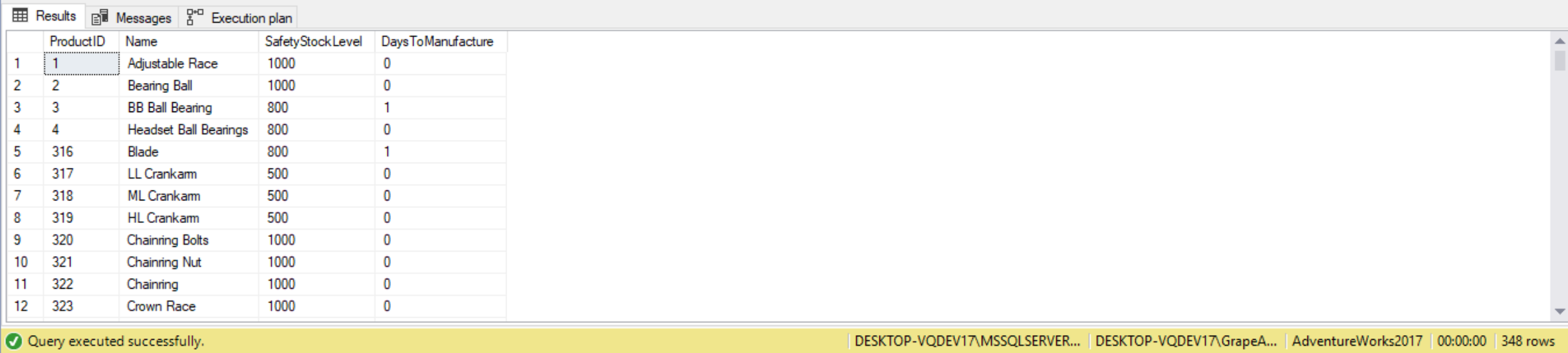
 When this subquery is run it first calculates the Average SafetyStockLevel. This returns a list of numbers. Then for each product row in the outer query SafetyStockLevel is compared. If it is greater than one or more from the list, then include it in the results. While ANY and MIN are equivalent in principle, we can’t use MIN, as shown by the error message from the following query:

SELECT ProductID, 
       Name, 
       SafetyStockLevel, 
       DaysToManufacture
FROM Production.Product
WHERE SafetyStockLevel > MIN(
(
    SELECT AVG(SafetyStockLevel)
    FROM Production.Product
    GROUP BY DaysToManufacture
));

 The ANY predicate can be substituted for the equivalent IN predicate. The same rules regarding the handling of NULLs apply.

The ALL modifier

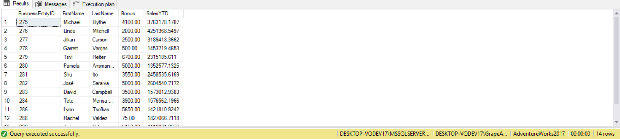
The ALL modifier works in similar fashion to ANY except it returns the outer row if its comparison value is greater than every value returned by the inner query. In other words, ALL is more restrictive in that all of the values in the subquery must satisfy the comparison condition. The comparison operator > ALL means greater than the MAX value of the list. In this example we’ll return all SalesPeople that have a bonus greater than ALL sales people whose year-to-date sales were less than a million dollars:

SELECT p.BusinessEntityID, 
       p.FirstName, 
       p.LastName, 
       s.Bonus, 
       s.SalesYTD
FROM Person.Person AS p
     INNER JOIN Sales.SalesPerson AS s ON p.BusinessEntityID = s.BusinessEntityID
WHERE s.Bonus > ALL
(
    SELECT Bonus
    FROM Sales.SalesPerson
    WHERE Sales.SalesPerson.SalesYTD < 1000000
);

 (Include TABLE from Wenzel)

The MAX aggregate function is used when we wish to find the highest value of something. The ALL predicate can accomplish the same thing. The MAX function discards NULLs and returns the first non-NULL record. With the ALL predicate, ALL literally means all. So if there is at least one NULL record, then the ALL predicate is FALSE because any comparison with FALSE is FALSE. The fix to this is to filter out any NULLs inside the inner query.

(Include code, explanation, similar to the ADVANCED BOOK)

Just like we can find use the ALL predicate to find the maximum value of something, we can also use it to find the minimum. Both the MAX and MIN functions discard NULL records, whereas ALL does not. Again, the fix to the issue would be filter out NULL records.

Even though MAX() vs >=ALL and MIN() vs >=ALL return identical rows (assuming no NULLs in the subquery), the performance can differ.

(Find example with execution plan)

Comparing Performance

(CONTINUE FROM ADVANCED BOOK/ PRIMER BLOG)

Using a subquery in a statement that modifies data

A subquery can be also be used within an INSERT, UPDATE or DELETE statement as well, like follows:

DECLARE @SQTable TABLE
(OrderID      INT, 
 OrderDate    DATETIME, 
 TotalDue     MONEY, 
 MaxOrderDate DATETIME
);
-- INSERT with SubQuery
INSERT INTO @SQTable
       SELECT SalesOrderID, 
              OrderDate, 
              TotalDue, 
       (
           SELECT MAX(OrderDate)
           FROM [Sales].[SalesOrderHeader]
       )
       FROM [Sales].[SalesOrderHeader]
       WHERE CustomerID = 29614;
-- Display Records
SELECT *
FROM @SQtable;

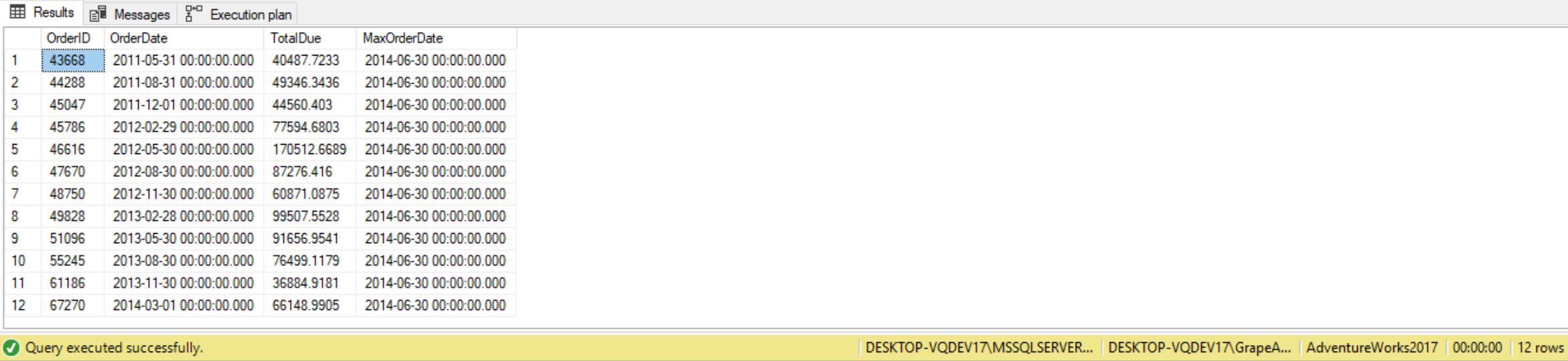
 Here, the subquery is used to calculate the value to be inserted into the column MaxOrderDate. This is only a single example of how to use a subquery in an INSERT statement. Keep in mind a subquery can be also be used within an UPDATE and/or DELETE statement as well.

Correlated subqueries can be used not only for returning a result set using a SELECT statement. We can also use them to update the data in a table. We first generate some test data in a tempdb table with the following code:

 

The code creates CarInventory table and then populates it with eight rows representing the cars currently in inventory.

We will write a query that will update the StickerPrice on all cars so each car with the same CarName value has the same InvoicePriceRatio. We want to set the StickerPrice to the same value as the maximum Sticker price for that CarName. This way all cars with the same CarName value will have the same StickerPrice value. To accomplish this update of the CarInventory table, we run the following code, which contains a correlated subquery.

USE tempdb;
GO
SET NOCOUNT ON;
CREATE TABLE CarInventory
(ID           INT IDENTITY, 
 CarName      VARCHAR(50), 
 VIN          VARCHAR(50), 
 StickerPrice DECIMAL(7, 2), 
 InvoicePrice DECIMAL(7, 2)
);
GO
INSERT INTO CarInventory
VALUES
('Explorer', 'EXP2014123456A', 46198.45, 38201.87),
('Explorer', 'EXP2014123493A', 47129.98, 38201.87),
('Grand Cherokee', 'JGC20141234345X', 41678.45, 36201.86),
('Grand Cherokee', 'JGC20141234556W', 44518.31, 36201.86),
('Pathfinder', 'NPF2014987365A', 32587.73, 28917.10),
('Pathfinder', 'NPF2014239657B', 33577.54, 28917.10),
('Pathfinder', 'NPF2014098587C', 35876.12, 28917.10),
('Tahoe', 'TAH201409674A', 52001.08, 46000.01);
SELECT * FROM CarInventory;

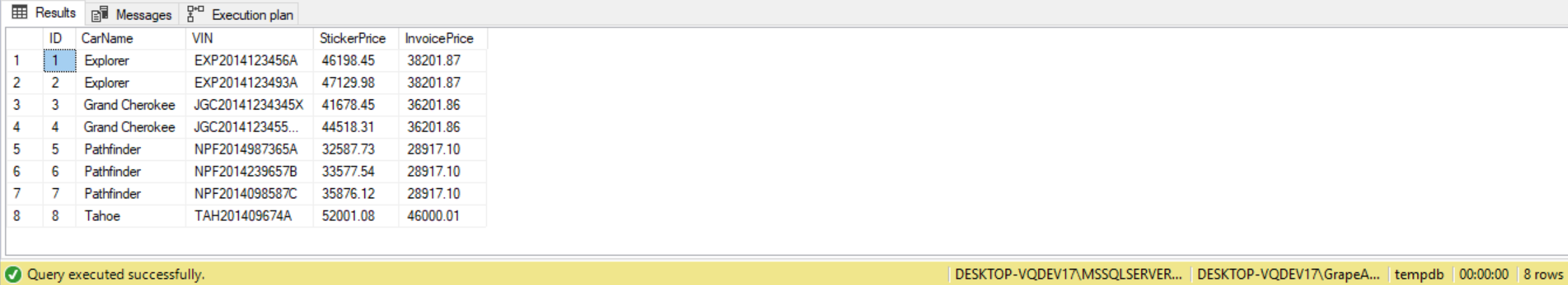
 The above uses the CarName from the outer query in the correlated subquery to identify the maximum StickerPrice for each unique CarName. This maximum StickerPrice value found in the correlated subquery is then used to update the StickerPrice value for each CarInventory record that has the same CarName.

Other Miscellaneous Considerations

• ntext, text and image data types are not allowed to be returned from a subquery.
• The ORDER BY clause cannot be used in a subquery unless the TOP operator is used.
• Views that use a subquery can’t be updated.
• COMPUTE and INTO clauses cannot be used in a subquery.