JOINs and Advanced JOINs
CROSS JOINS
- Self-Cross Joins
- The Dating Service Scenario
- Producing tables of numbers
- INNER JOIN as CROSS JOIN
- Performance Considerations
INNER JOINs
- Inner joins syntax
- Join Query Table Order
More join examples:
- Composite joins
- Non-equi joins
- Non-equi join to calculate running total
- Non-equi join to check for duplicate values
- Non-equi join to compare a range of values
- The Salary Levels Scenario
- Multi-join queries
OUTER JOINS
- Fundamentals of Outer Joins
- Beyond the fundamentals of Outer Joins
- Introducing missing values
- Filtering attributes from the nonpreserved side of an outer join
- Using outer joins in a multi-join query
- Using the COUNT aggregate with outer joins
Using JOINs to Modify Data
- Using joins to delete data
- Using joins to update data
Performance Considerations
- Completely Qualified Filter Criteria
- Join Hints
- Performance Guidelines
(INCLUDE SYNTAX WITH EVERYTHING)
(INCLUDE NOTES FROM PRAGMATIC WORKS INTRO AND ADVANCED, DATABASESTAR ACADEMY, SQL COOKBOOK, ABSTRACTSQLENGINEER, WENZEL)
(COMPARE WITH ADVANCED SQL BOOK ONE LAST TIME)
(ALSO CHECK OUT JOINS DIAGRAM FOR BLOG EMAIL)
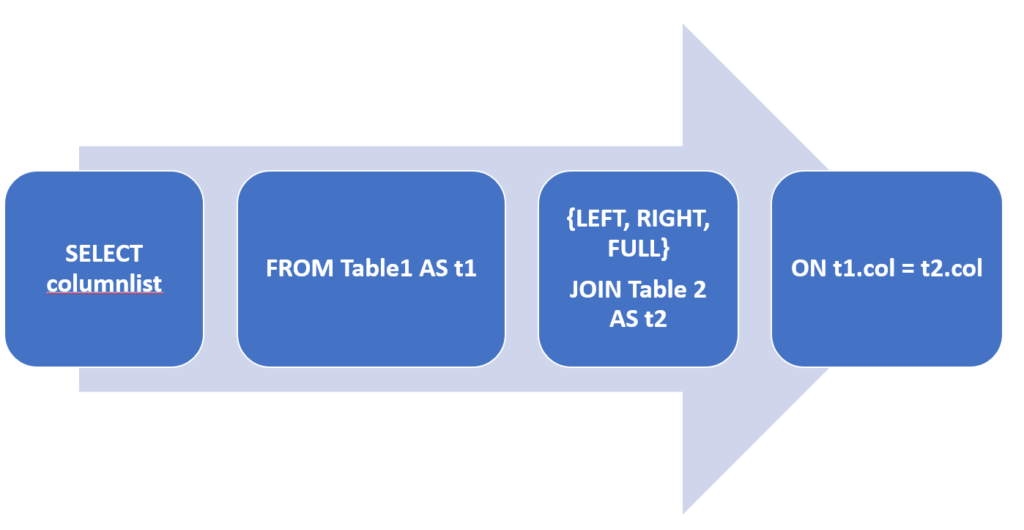
JOINs
T-SQL supports four different table operators: JOIN, APPLY, PIVOT, and UNPIVOT. Out of the four, only JOIN is ANSI-standard while the other three are T-SQL extensions. Table operators accept tables as input, apply some logical query processing, and return a table result set.
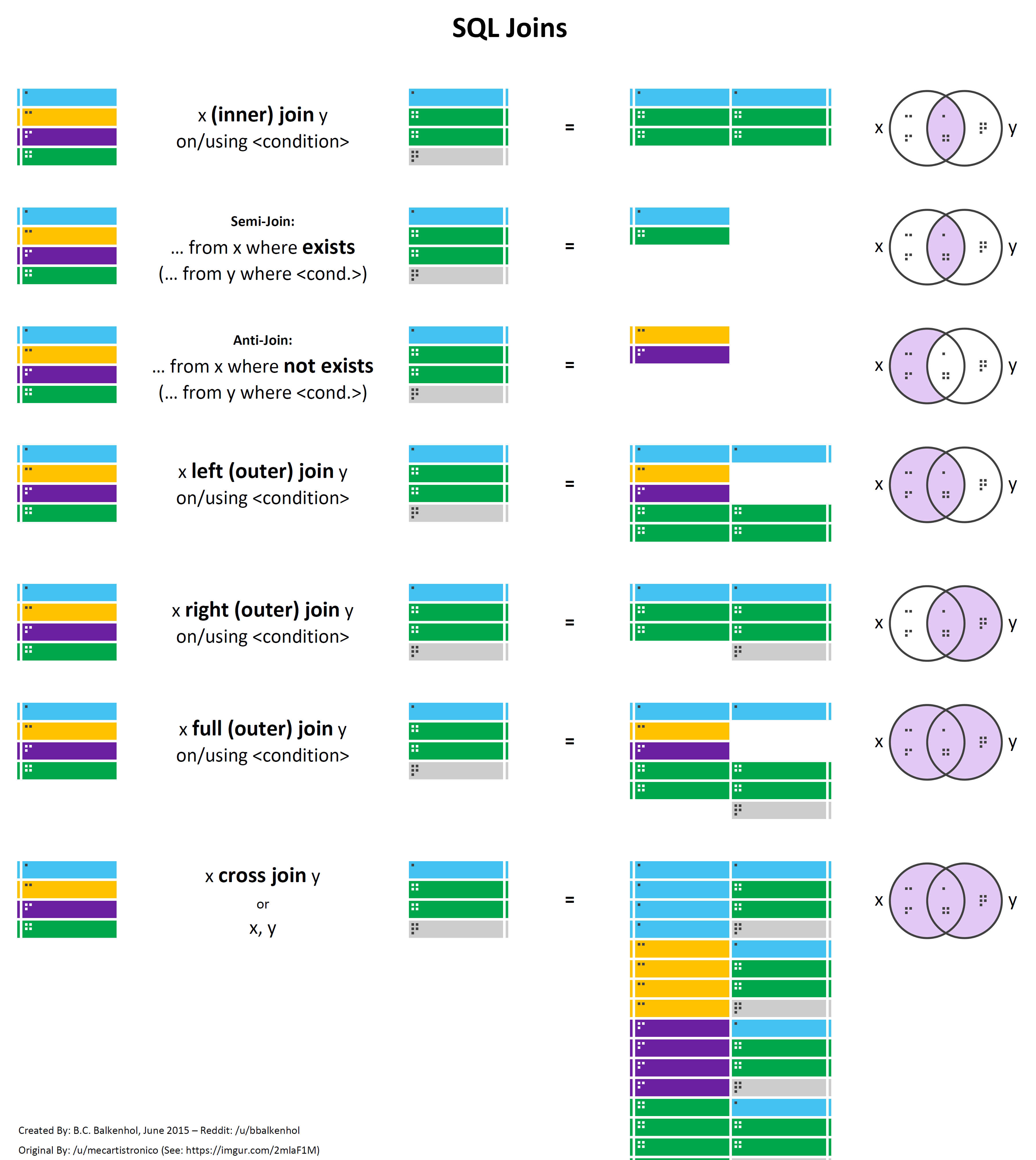
The JOIN table operator accepts two tables as input. The three main types of joins in T-SQL include CROSS JOINs, INNER JOINs, and OUTER JOINs (Left, Right, and Full).
CROSS JOINs
(Include notes from Joes2Pros, AbstractSQLEngineer, SQL Cookbook, Vertabelo Academy, 70-461 book, and Udemy ‘SQL Server Essentials’)
(Verify Ben Brumm)
(In addition to Ben Brumm verify- Join without the ON condition is not best practice. Instead, it is best practice to specifiy the CROSS JOIN Keyword)
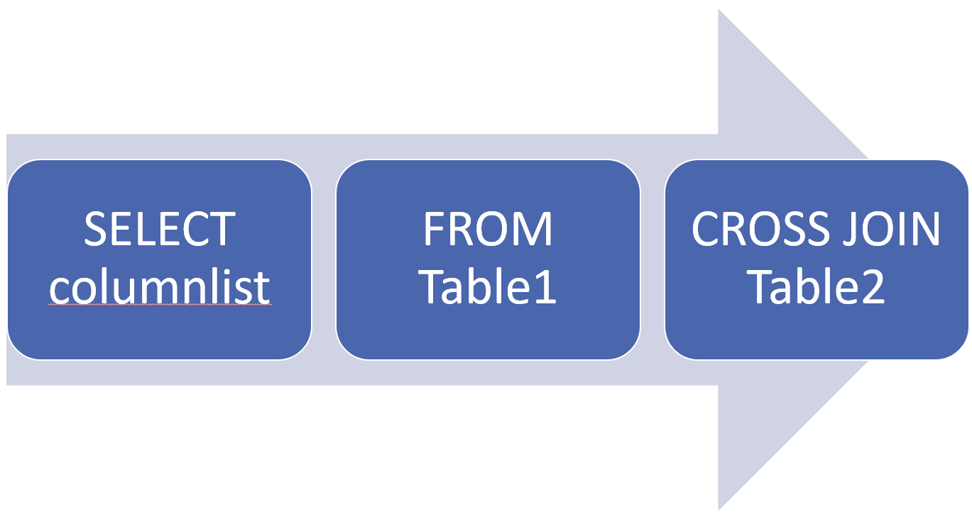
The CROSS JOIN returns all possible combinations of every row from two tables. Cross joins implement only one logical query processing phase- a Cartesian product. Join conditions aren’t used with cross joins, meaning no matching is performed on columns. It accepts two tables as input to return a table representing a Cartesian product of the two input tables. In other words, each row from one table is matched with all rows from the other table. So, if we have m rows in one table and n rows in the other, the result set table will contain m * n rows. In other words, if no filter is used, the number of rows in the result set is the number of rows in one table multiplied by the number of rows in the other table. A common use case for a cross join is to generate data derived from combinations of items, such employees and dates representing workdays when the employee and dates columns are each living in different tables. The CROSS JOIN keyword is used to define a cross join:
As an example, the following query applies a cross join between the Sales.Customer and HumanResources.Employee table in the AdventureWorks2017 database, returning all possible combinations of CustomerID and BusinessEntityID attributes in the result set:
USE AdventureWorks2017;
SELECT c.CustomerID,
       e.BusinessEntityID
FROM SALES.Customers AS c
     CROSS JOIN HumanResources.Employee AS e;
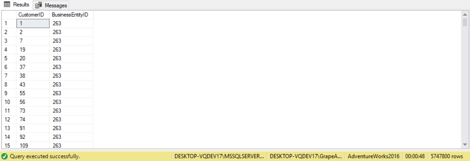
There are 19,820 rows in the Sales.Customer table and 299 rows in the HumanResources.Employee table, so the result set contains 5,747,800 rows (19820 * 290 = 5747800). This combinatoric effect make cross joins extremely dangerous! This is because cross joins may have poor performance when the tables involved are massive, since SQL Server will require a lot of time and resources to return the result set.
Note that the Sales.Customer and HumanResources.Employee table are given aliases of c and e, respectively. These aliases are used as prefixes for the columns used in the join condition. These prefixes do not appear in the final query result. If no aliases are assigned to the input tables, then the names of the table would serve as the prefixes in the join condition instead. We use prefixes in the join condition so that the columns are identified in an unambiguous manner when both tables have the same column name. Aliasing the tables allows for brevity for large input table names. Column prefixes are required when referring ambiguous column names (ie. the two input tables have the same column name). Use of column prefixes is optional for unambiguous cases. For the sake of clarity, it’s good practice to always use column prefixes. Once we assign an alias to a table, it’s invalid to use the full table name as a column prefix.
Another example of a CROSS JOIN:
--CROSS JOIN: A JOIN without an ON condition
--FirstName repeated once for every date in the second result set
USE AdventureWorksDW2016
SELECT de.EmployeeKey,
       FirstName,
       dd.FullDateAlternateKey
FROM DimEmployee AS de
     CROSS JOIN DimDate AS dd
WHERE dd.FullDateAlternateKey BETWEEN '1/1/2008' AND '1/10/2008'
ORDER BY EmployeeKey;
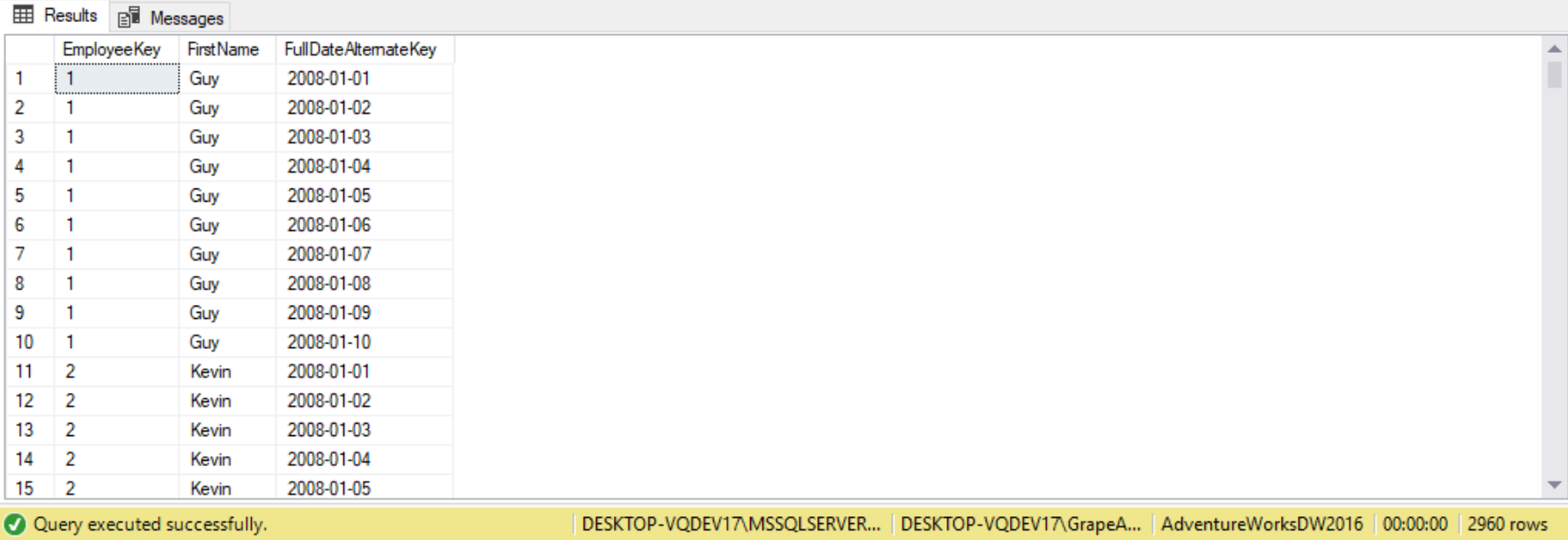
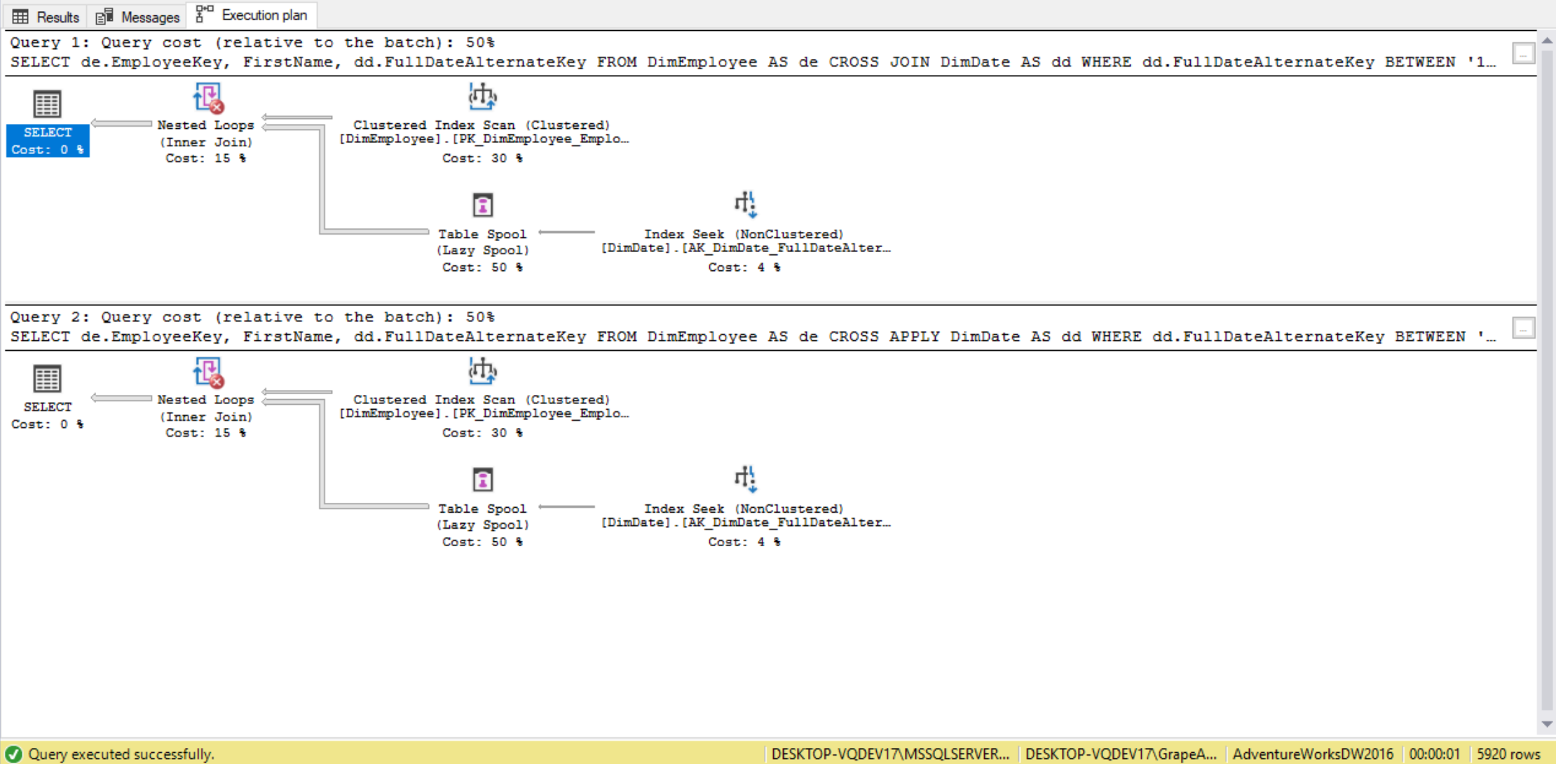
Notice that each FirstName is repeated 10 times, since the date filter returns 10 dates. Since we have 2960 returned records, we actually have 296 first names.
Using CROSS APPLY will return the exact same result set. The execution plan is the exact same as well:
--FirstName repeated once for every date in the second result set that we're doing CROSS JOIN to
SELECT de.EmployeeKey,
       FirstName,
       dd.FullDateAlternateKey
FROM DimEmployee AS de
     CROSS APPLY DimDate AS dd
WHERE dd.FullDateAlternateKey BETWEEN '1/1/2008' AND '1/10/2008'
ORDER BY EmployeeKey;
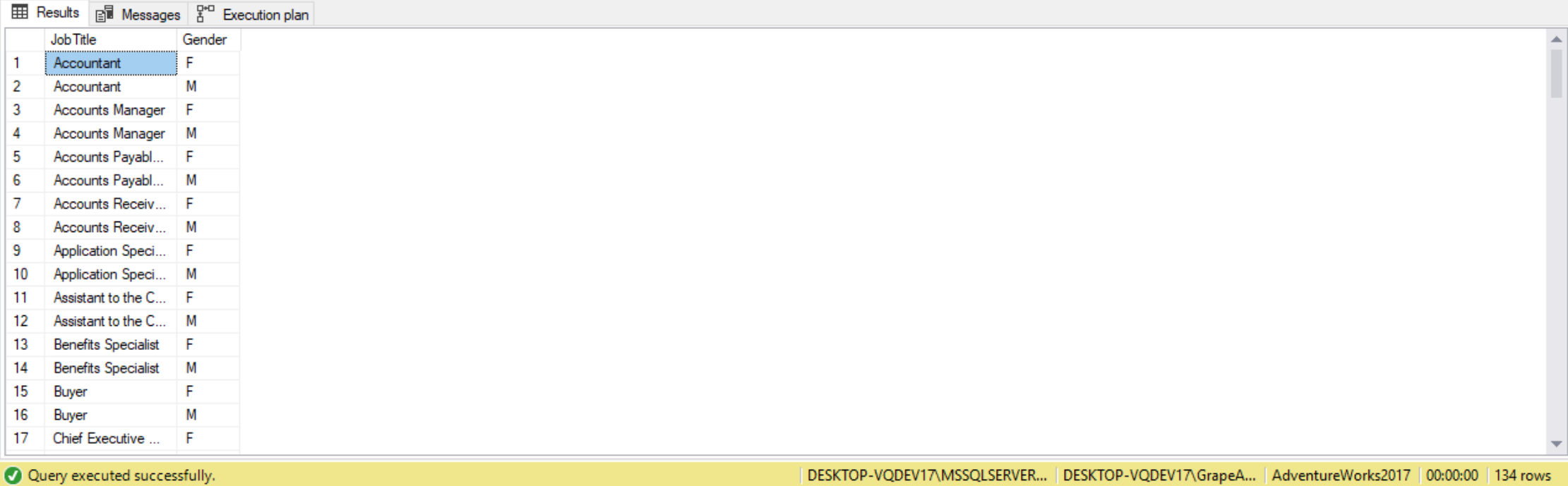
For another example, let’s suppose we wish to return the number of employees for each title, grouped by gender, even if there is only 1 gender for a particular title. To get a combination of JobTitle and Gender even when the count is zero, we can use a cross join. The following are the steps we can take to create the result.
- Create a CTE (Common Table Expression) to get a distinct list of JobTitles.
- Create a CTE to get a distinct list of Genders.
- Create a CTE to compute a summary count of employees by JobTitle and Gender.
- Use a CROSS JOIN to create a distinct list of all possible combinations of JobTitles and Genders.
- Take the result set from Step 5 and LEFT OUTER JOIN that to the CTE with the summary count on their respective JobTitle and Gender The outer join will return the cross joined result set even for records where there is no match between the outer joining tables. The COALESCE function is used to replace NULLs (in the case for non-matching records) with a zero value.
The query would be as follows:
USE AdventureWorks2017
;WITH cteJobTitle(JobTitle)
     AS (SELECT DISTINCT
                JobTitle
         FROM HumanResources.Employee),
     cteGender(Gender)
     AS (SELECT DISTINCT
                Gender
         FROM HumanResources.Employee)
     SELECT J.JobTitle,
            G.Gender
     FROM cteJobTitle AS J
          CROSS JOIN cteGender AS G
     ORDER BY J.JobTitle;
(Include example and code from the Stairways series under “Using CROSS JOIN to find products not sold”)
We can use the CROSS JOIN operator to perform a cross join operation across multiple tables. The following query is an example:
(Include code, explanation, and results from Stairway Series)
Self cross joins
There are some situations where we need to join a table to itself . A self join is when we join multiple instances of the same table. Self joins are supported with cross joins, inner joins, and outer joins. For example, the following code queries a self cross join between two instances of the HumanResources.vEmployee table:
SELECT e1.BusinessEntityID,
       e1.FirstName,
       e1.LastName,
       e2.BusinessEntityID,
       e2.FirstName,
       e2.LastName
FROM HumanResources.vEmployee AS e1
     CROSS JOIN HumanResources.vEmployee AS e2;
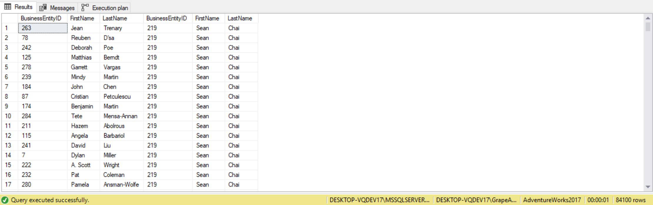
Since the HumanResources.vEmployee table has 290 rows, the query returns 84,100 rows (290 * 290 = 84100) representing all possible combinations of pairs of employees.
In a self-join, aliasing the tables is required to ensure the column names in the join condition are unambiguous.
The Dating Service Scenario
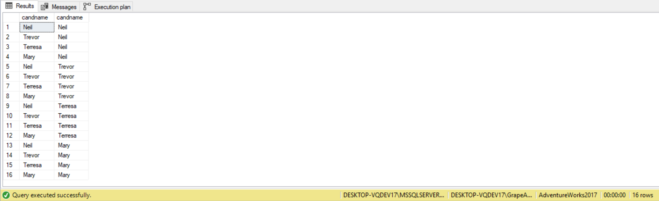
Suppose we have a database for a dating service, containing a table with the name of the candidates and their gender. We need to match all possible candidates, so for this particular example, the request is to match males with females.
The code to create our demo table is as follows:
CREATE TABLE candidates
  (
     candname VARCHAR(10) NOT NULL,
     gender   CHAR(1) NOT NULL CONSTRAINT chk_gender CHECK (gender IN('F', 'M'))
  )

INSERT INTO candidates
VALUES     ('Neil',
            'M')

INSERT INTO candidates
VALUES     ('Trevor',
            'M')

INSERT INTO candidates
VALUES     ('Terresa',
            'F')

INSERT INTO candidates
VALUES     ('Mary',
            'F')
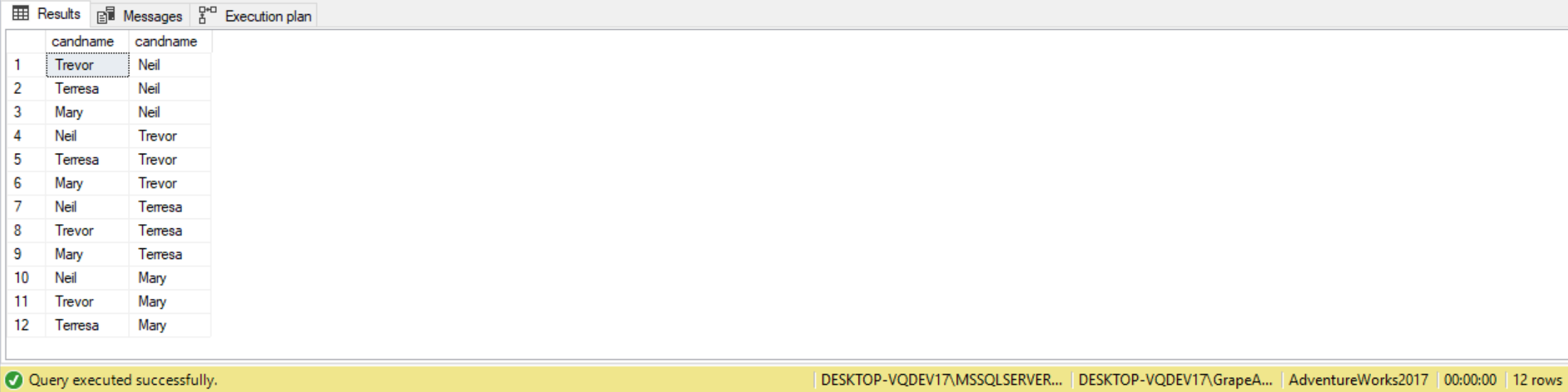
Let’s first write a CROSS JOIN query:
SELECT T1.candname,
       T2.candname
FROM   candidates AS T1
       CROSS JOIN candidates AS T2
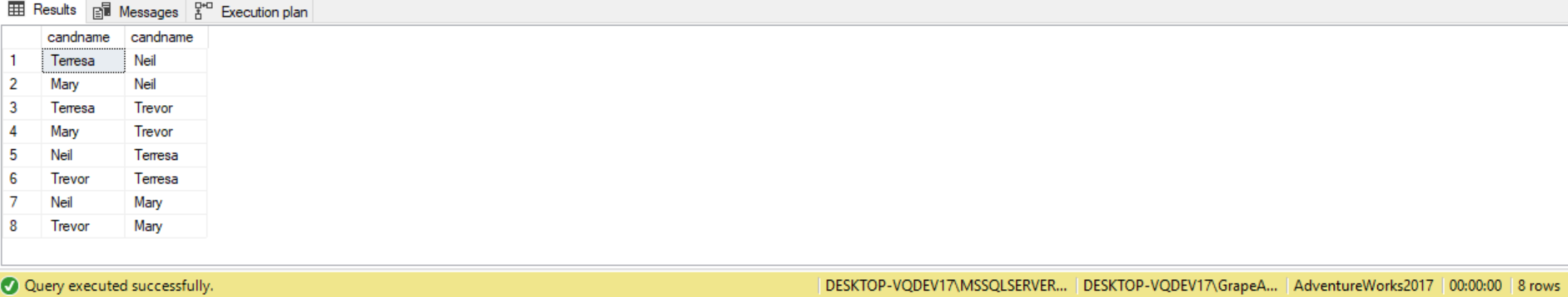
Now, we don’t want anyone go on a date with themselves, so here is a modification to the query:
SELECT T1.candname,
       T2.candname
FROM   candidates AS T1
       CROSS JOIN candidates AS T2
WHERE  T1.candname <> T2.candname
Since we’re trying to match males with females, we need to eliminate couples with the same gender. Here’s how the query would go:
SELECT T1.candname,
       T2.candname
FROM   candidates AS T1
       CROSS JOIN candidates AS T2
WHERE  T1.gender <> T2.gender
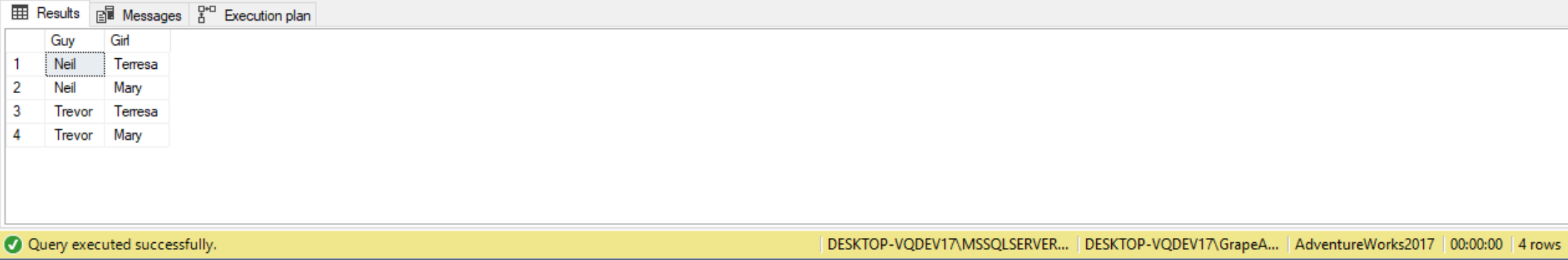
Finally, we need to remove duplicates since we don’t wish the couple going on a date twice. We do this by requesting a specific gender for each column, as shown below:
SELECT M.candname AS Guy,
       F.candname AS Girl
FROM   candidates AS M
       CROSS JOIN candidates AS F
WHERE  M.gender <> F.gender
       AND M.gender = 'M'
We can also use one condition that takes care of all problems, as follows:
SELECT M.candname AS Guy,
       F.candname AS Girl
FROM   candidates AS M
       CROSS JOIN candidates AS F
WHERE  M.gender > F.gender
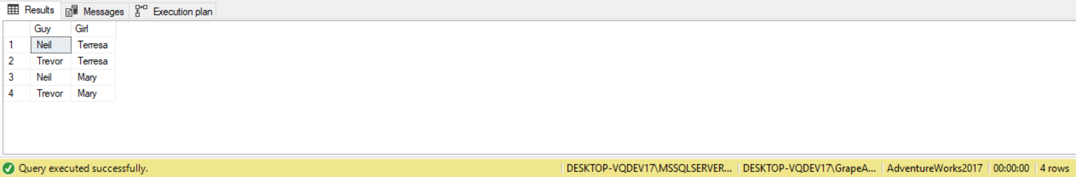
Here, nobody dates himself or herself, the genders are different, and since the letter M is higher than the letter F, we ensure that only males appear in the first column.
Producing tables of numbers
A common use case for cross joins is when they are used to produce a result set with a sequence of numbers (1,2,3, and so on). Using cross joins allows us to produce the sequence of integers in a very efficient manner.
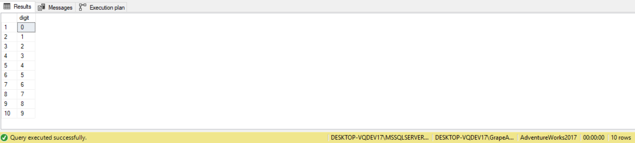
For example, in the following code we’re creating a table called Digits having a column called digits. Using the INSERT statement, this table is populated with 10 rows containing the digits 0 through 9:
USE AdventureWorks2017;

DROP TABLE IF EXISTS dbo.Digits;

CREATE TABLE dbo.digits(digit INT NOT NULL PRIMARY KEY);

INSERT INTO dbo.digits(digit)
VALUES(0), (1), (2), (3), (4), (5), (6), (7), (8), (9);

SELECT digit FROM dbo.Digits;
Similar to the above query, we can use cross joins to create a sequence of integers in the range 1 through 1000. We apply cross joins between three instances of the Digits table, each representing a different power of 10 (1,10,100). By multiplying three instances of the same table, we get returned a result set containing 1000 rows (10*10*10=1000). To produce the sequence of numbers, we then multiply the digit from each instance by the power of 10 it represents (1,10,100), sum the results and then add 1 to those, like follows:
SELECT d3.digit * 100 + d2.digit * 10 + d1.digit + 1 AS n
FROM dbo.Digits AS d1
     CROSS JOIN dbo.Digits AS d2
     CROSS JOIN dbo.Digits AS d3
ORDER BY n;
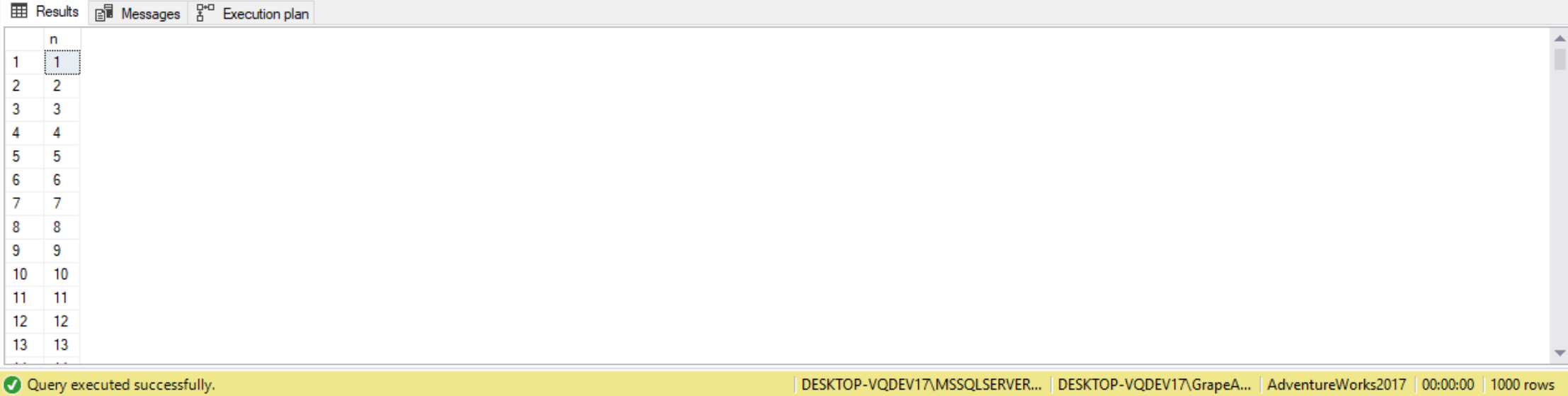
The above query is how we can return a sequence of 1000 integers. Similarly, to produce a sequence of 1000000 rows, we apply cross joins to six instances of the Digits table.
INNER JOIN as CROSS JOIN
There is a way to use the WHERE clause to have a CROSS JOIN behave like an INNER JOIN. When we use a WHERE clause that constrains the joining of the tables in a cross join, SQL Server doesn’t create a Cartesian product but instead functions like a normal join operation. Suppose we wish to birth date and last name for all employees. To accomplish this, we need to relate the Employee and Person tables.
SELECT P.LastName,
       E.BirthDate
FROM HumanResources.Employee E
     CROSS JOIN Person.Person P;
This query isn’t useful as it is returning nearly 6 million rows! To limit the row combinations so that the records from the Person table is properly matched with records from the Employee table, we can use a where clause, like follows:
SELECT P.LastName,
       E.BirthDate
FROM HumanResources.Employee E
     CROSS JOIN Person.Person P
WHERE P.BusinessEntityID = E.BusinessEntityID;
We not get returned 290 rows. This query will return the same results as one using an INNER JOIN. The inner join equivalent of the above query is as follows:
SELECT P.LastName,
       E.BirthDate
FROM HumanResources.Employee E
     INNER JOIN Person.Person P ON P.BusinessEntityID = E.BusinessEntityID;
If we look at the query plans, we’ll see the two queries are very similar:
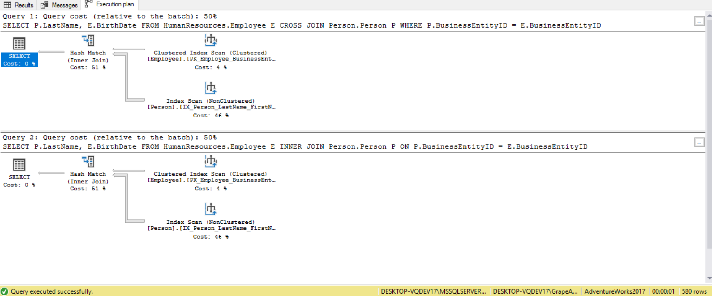
In this case, the query plans are identical. This is because SQL is a declarative language, and the SQL Server optimizer will re-write the query when a CROSS JOIN operation is used in conjunction with a WHERE clause that provides a join predicate between the two join tables involved in the CROSS JOIN. In most cases the SQL Server engine generates the same execution plan.
Performance Considerations
Because a CROSS JOIN joins every record from one table to every row on another table, the result set can become very large. For example, if we cross join a table with 1,000,000 rows with another table with 100,000 rows, we get returned a result set containing 100,000,000,000 rows, and will take SQL Server a lot of time to create it. When using cross joins, we should try to minimize the size of the tables being cross joined if we want to optimize the performance. The following code generates a table for our next demo:
CREATE TABLE Cust (Id int, CustName varchar(20));
CREATE TABLE Sales (Id int identity
                    ,CustID int
					,SaleDate date
					,SalesAmt money);
SET NOCOUNT ON;
DECLARE @I int = 0;
DECLARE @Date date;
WHILE @I < 1000
BEGIN
	SET @I = @I + 1;
	SET @Date = DATEADD(mm, -2, '2014-11-01');
	INSERT INTO Cust
	VALUES (@I,
	        'Customer #' + right(cast(@I+100000 as varchar(6)),5));
	WHILE @Date < '2014-11-01'
	BEGIN
		IF @I%7 > 0
			INSERT INTO Sales (CustID, SaleDate, SalesAmt)
			VALUES (@I, @Date, 10.00);
		SET @Date = DATEADD(DD, 1, @Date);
	END
END
The code above creates 2 months’ worth of data for 1,000 different customers. The code adds no sales data for the 7th customer. The Cust table has 1,000 rows while the Sales table has 52,338 rows. The following two queries are used to demonstrate how the CROSS JOIN operator performs differently depending on the sizes of the tables involved:
SET STATISTICS IO, TIME ON;

SELECT CONVERT(CHAR(6), s1.SaleDate, 112) AS SalesMonth,
       s.CustName,
       ISNULL(SUM(s2.SalesAmt), 0) AS TotalSales
FROM   Cust c
       CROSS JOIN (SELECT SaleDate
                   FROM   Sales) AS s1
       LEFT OUTER JOIN Sales AS s2
                    ON c.id = c2.CustID
                       AND s1.SaleDate = s2.SaleDate
GROUP  BY CONVERT(CHAR(6), s1.SaleDate, 112),
          c.CustName
HAVING ISNULL(SUM(s2.SalesAmt), 0) = 0
ORDER  BY CONVERT(CHAR(6), s1.SaleDate, 112),
          c.CustName
SET STATISTICS IO, TIME ON;

SELECT CONVERT(CHAR(6), s1.SaleDate, 112) AS SalesMonth,
       c.CustName,
       ISNULL(SUM(s2.SalesAmt), 0) AS TotalSales
FROM   Cust c
       CROSS JOIN (SELECT DISTINCT SaleDate
                   FROM   Sales) AS s1
       LEFT OUTER JOIN Sales s2
                    ON c.Id = s2.CustId
                       AND s1.SaleDate = s2.SaleDate
GROUP  BY CONVERT(CHAR(6), s1.SaleDate, 112),
          c.CustName
HAVING ISNULL(SUM(s2.SalesAmt), 0) = 0
ORDER  BY CONVERT(CHAR(6), s1.SaleDate, 112),
          c.CustName
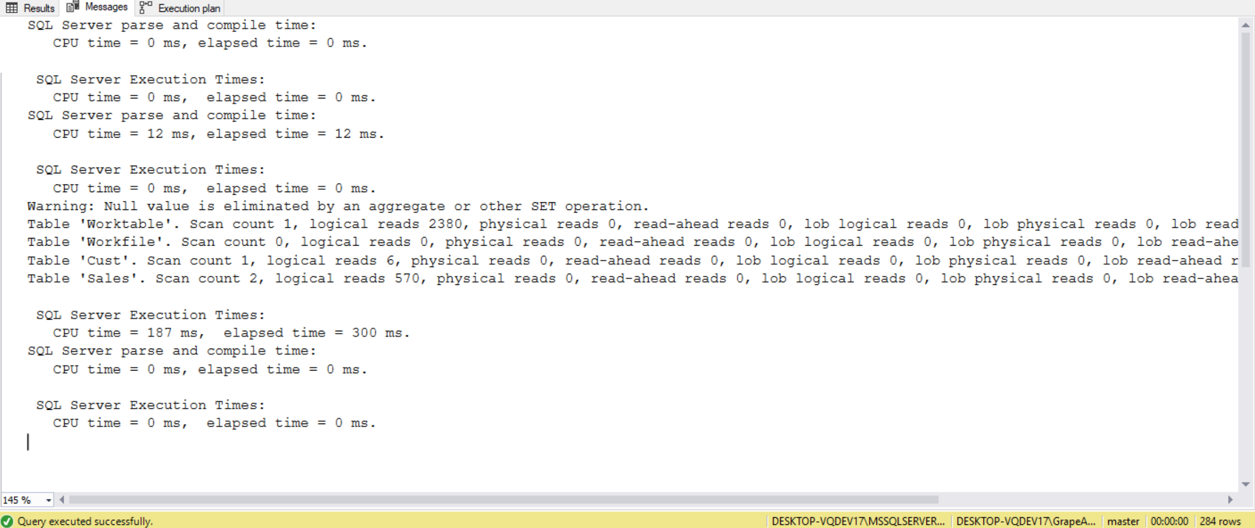
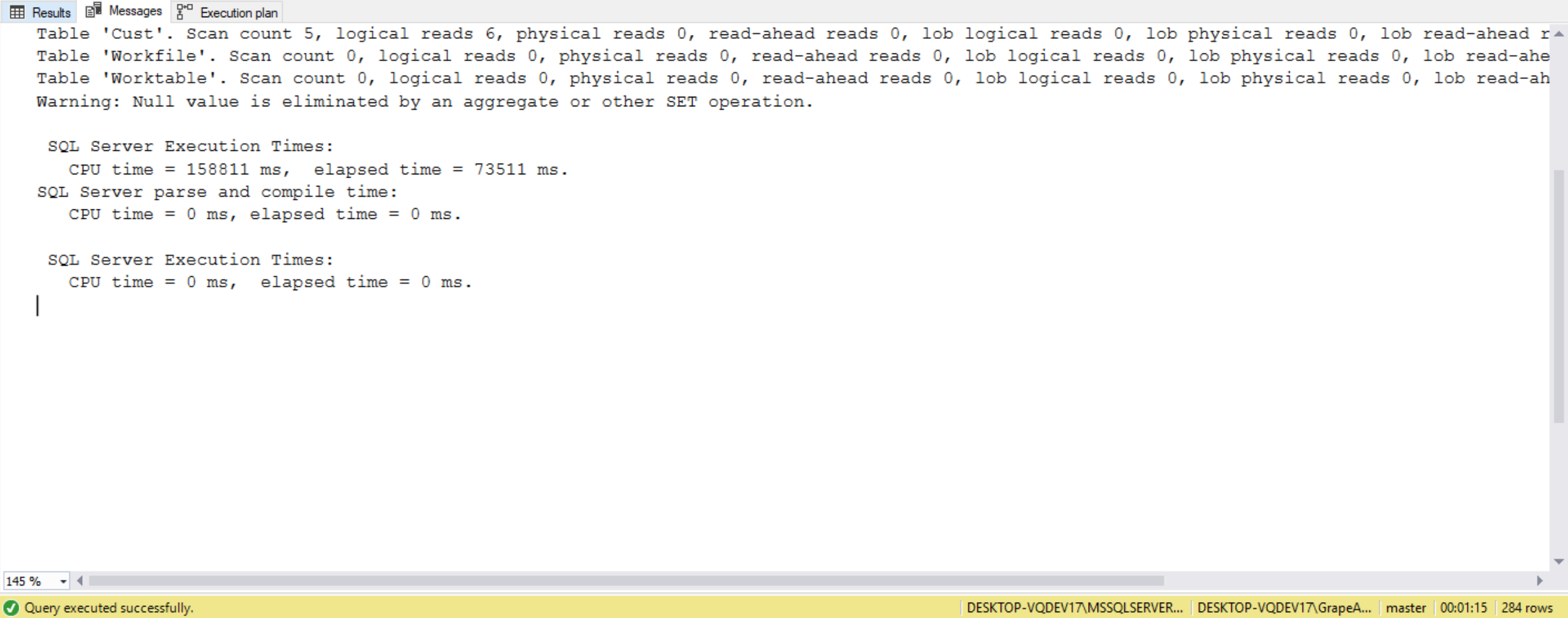
In the first query, we cross join the Sales (52,338 rows) and Cust (1,000 rows) tables to return 52,338,000 rows, which is then used to determine the customers with zero sales in a month. In the second query, we change the selection criteria from the Sales table to only return a distinct set of SalesData values. This distinct set returns only 61 different SalesData values, which is cross joined to the Cust table to now return 61,000 rows. By reducing the size of records returned from the Sales table we were able to execute the query to less than 1 second, whereas the first query took 19 seconds to complete (VERIFY THIS!). The execution plans for the two queries are slightly different from each other. The estimated number of records generated from the Nested Loops (Inner Join) operation on the right side of the graphical plan is 52,338,00 records for the first query, whereas the same operation for the second query estimates 61,000 records. The large result set from the first query’s plan generated from the CROSS JOIN Nested Loops operation is then passed through to several additional operations. Because all these operations in the first query has to work against 52 million records, it is substantially slower than the second query. Therefore, the number of records used in a CROSS JOIN operation dramatically affect the length of time a query runs. If we write our query to minimize the number of records involved in the CROSS JOIN operation, our query will perform much more efficiently.
(Include execution plans for both queries from Stairway Series)
Inner joins
(Include notes from Joes2Pros, Udemy SQL, AbstractSQLEngineer, SQL Cookbook, Vertabelo Academy, 70-461 book, and Udemy ‘SQL Server Essentials’)
The INNER JOIN returns only records that are matching on both tables. Rows that match remain in the result, and those that don’t are rejected. A common situation for inner joins is where we need to join the primary key of one table to the foreign key of another. The inner join involves two logical querying processes: it first applies a Cartesian product between two input tables like a cross join, and then it filters the rows based on a specified predicate.
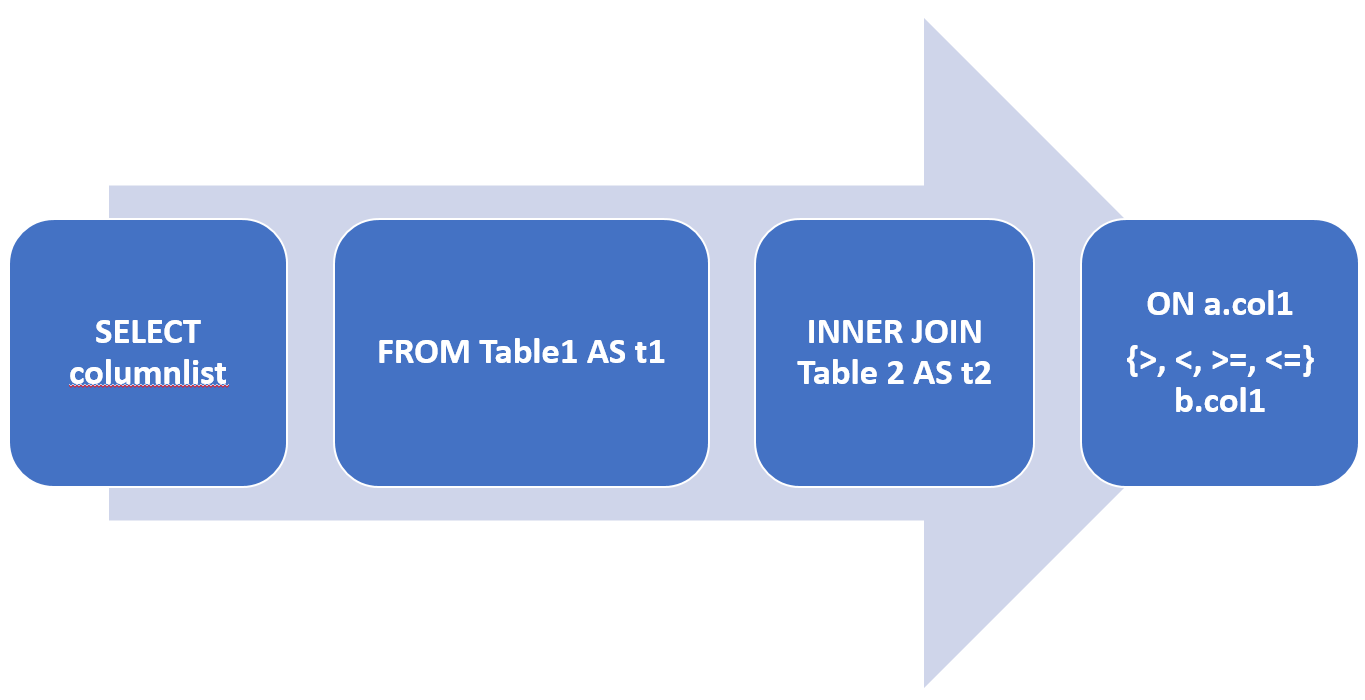
Inner Joins Syntax
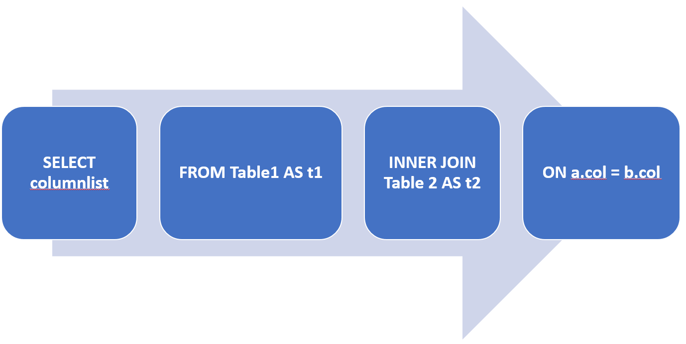
When applying an inner join, we specify the INNER JOIN keyword between the two input table names. The INNER keyword is optional, since the inner join is the default in SQL. The ON clause is used to specify the predicate used to filter the rows, also known as the join condition.
Where a same column name exists in two (or more) tables, and the column is the primary key on one table, and a foreign key on another, we must specify if we want CustomerID from Sales.Customer table, or CustomerID from the Sales.SalesOrderHeader table, for instance.
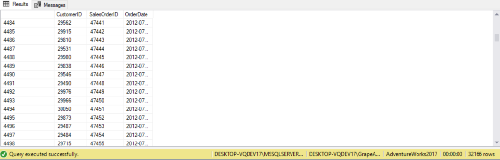
As an example, the following query applies an inner join between the Sales.Customer and Sales.SalesOrderHeader tables in the AdventureWorks2017 database, returning matching records based on the join condition c.CustomerID=soh.CustomerID:
USE AdventureWorks2017;
SELECT c.CustomerID,
       c.AccountNumber,
       soh.SalesOrderID,
       soh.OrderDate
FROM Sales.Customer AS c
     INNER JOIN Sales.SalesOrderHeader AS soh ON c.CustomerID = soh.CustomerID;
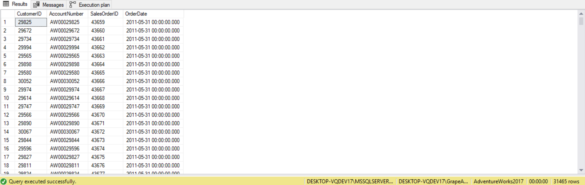
Inner joins can be imagined in terms of relational algebra. The query first applies a Cartesian product between the Sales.Customer and Sales.SalesOrderHeader tables, resulting in 51,285 rows (19820 Sales.Customer rows * 31465 Sales.SalesOrderHeader rows). Then the predicate c.CustomerID=soh.CustomerID is used by the join to filter rows, returning 31,465 records. While this is the logical way the inner join is processed, the physical processing of the query by the database engine can be different in practice.
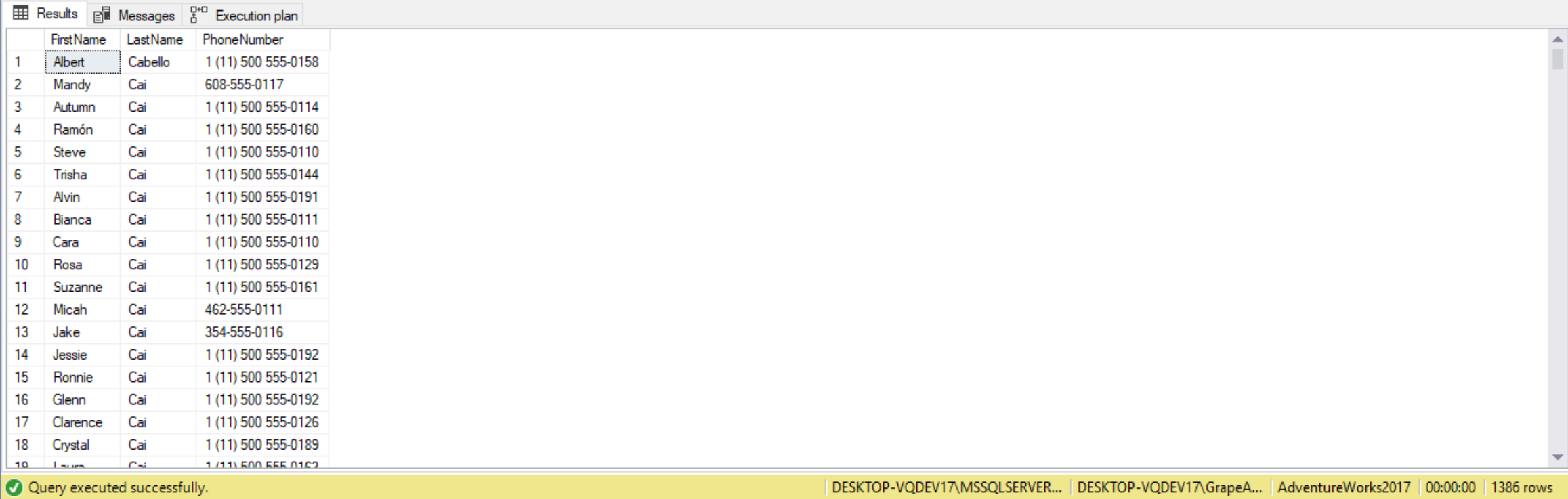
Once the data is joined it can also be filtered and sorted using the WHERE and ORDER BY clauses. The WHERE clause can refer to any of the fields from the joined tables. It’s best practice to prefix the columns with the table name or alias. The same goes for sorting. Any field can be used, but it’s common practice to sort by one or more fields in the SELECT list. For example, the following query with list people, in order of their last name, whose last name starts with C:
SELECT    Person.FirstName,
          Person.LastName,
          PersonPhone.PhoneNumber
 FROM     Person.Person
          INNER JOIN
          Person.PersonPhone
          ON Person.BusinessEntityID =
             PersonPhone.BusinessEntityID
 WHERE    Person.LastName LIKE 'C%'
 ORDER BY Person.LastName
Just like with the WHERE and HAVING clauses, the ON clause also returns only records for which the predicate evaluates to TRUE. Any rows evaluating to FALSE or UNKNOWN are discarded. So, any employees with no related orders will be discarded. The same is the case for orders with no related employees, but in this case the foreign-key relationship forbids these in our sample TSQLV4 database.
--Inner JOIN based on two JOIN criterias
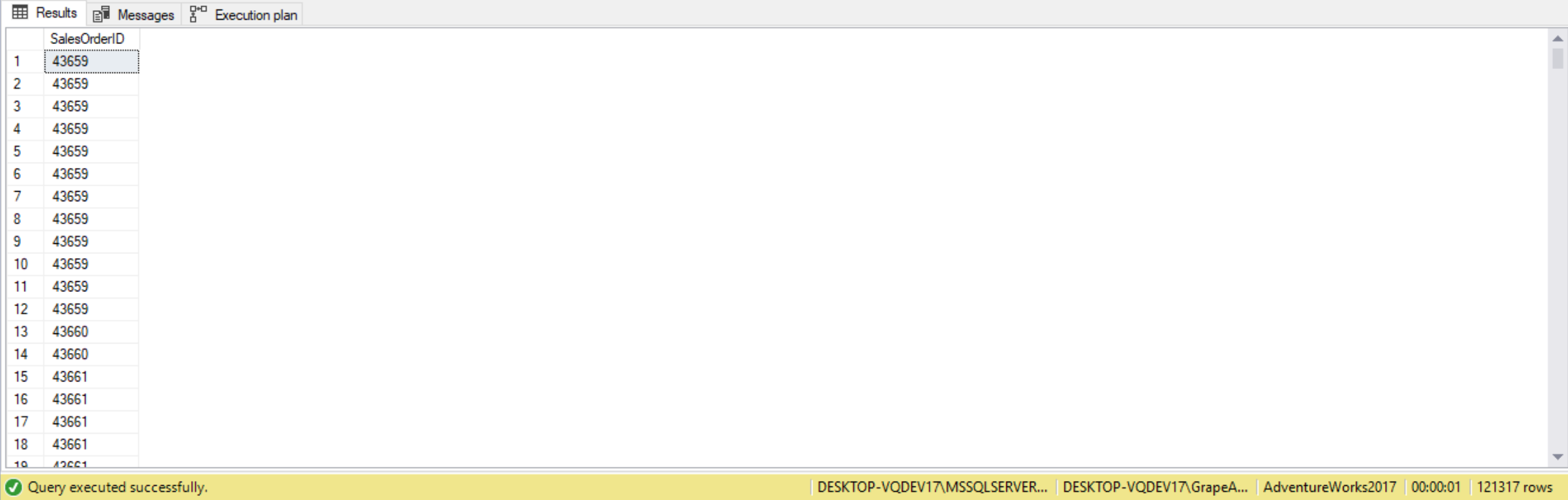
SELECT sod.SalesOrderID
FROM Sales.SalesOrderDetail AS sod
INNER JOIN Sales.SpecialOfferProduct AS sop
ON sod.ProductID = sop.ProductID
AND sod.SpecialOfferID = sop.SpecialOfferID;
Note that ANSI standard SQL supports the natural join. A natural join is an inner join between two tables on columns having the same name. For example, “T1 NATURAL JOIN T2” joins the tables T1 and T2 based on the column with the same name on both sides. T-SQL does not support natural joins.
A self join is when we inner join a table to itself. When we use a self-join it is important to alias the table. Suppose we wanted to list all departments within a department group. In the AdventureWorks2017 database, this query would go as follows:
SELECT  D1.Name,
        D2.Name
 FROM   HumanResources.Department AS D1
        INNER JOIN
        HumanResources.Department AS D2
        ON d1.GroupName = d2.GroupName

A join will match as many rows as it can between tables. Typically joining two or more fields happens when a table’s primary key consists of two or more columns. This is easily done using an AND operator and an additional join condition. When joining on more than one field, it’s important to understand each table’s primary key definition and to know how tables’ are meant to relate to one another.
(Make up an example using AdventureWorks2017)
Join Query Table Order
In the case of inner joins involving more than two tables, it doesn’t matter in which order the tables appear in the query. The performance and output of the query would be the same. The query processor will decide on the internal order in which it accesses the tables based on cost estimation, and it will come up with the same execution plan regardless of the order of the tables in the query. With joins involving more than two tables, the order of the tables in the query may produce different results, and therefore might require a different execution plan. If we were testing the performance of a query and would like to see the effects of forcing a specific join order, we can add to the query an OPTION clause that contains a FORCE ORDER hint, as shown here:
(Include code, explanation, and result from page 24 of ADVANCED BOOK)
Suppose in the AdventureWorks2017 database we need to join to the PhoneNumberType to know whether a listed phone number is a home, cell, or office number. By adding another INNER JOIN clause, we can create a directory of names, phone number types, and numbers by joining three tables together. The query would go as follows:
SELECT    C.Instructor,
          C.ClassName,
          S.Day,
          S.Hour
 FROM     Class AS C
          INNER JOIN
          Section AS S
          ON C.ClassName = S.ClassName
             AND C.Instructor = S.Instructor
          ORDER BY C.Instructor, S.Day, S.Hour
Suppose we’re using the HumanResources database, and we wish to return employee and department information, as well as job information from a third table. Here’s how the query would go:
--Three table JOIN
SELECT c.CustomerID,
       c.AccountNumber,
       soh.SalesOrderID,
       soh.OrderDate,
       sod.ProductID,
       sod.OrderQty
FROM Sales.Customer AS c
     INNER JOIN Sales.SalesOrderHeader AS soh ON c.CustomerID = soh.CustomerID
     INNER JOIN Sales.SalesOrderDetail AS sod ON soh.SalesOrderID = sod.SalesOrderID;
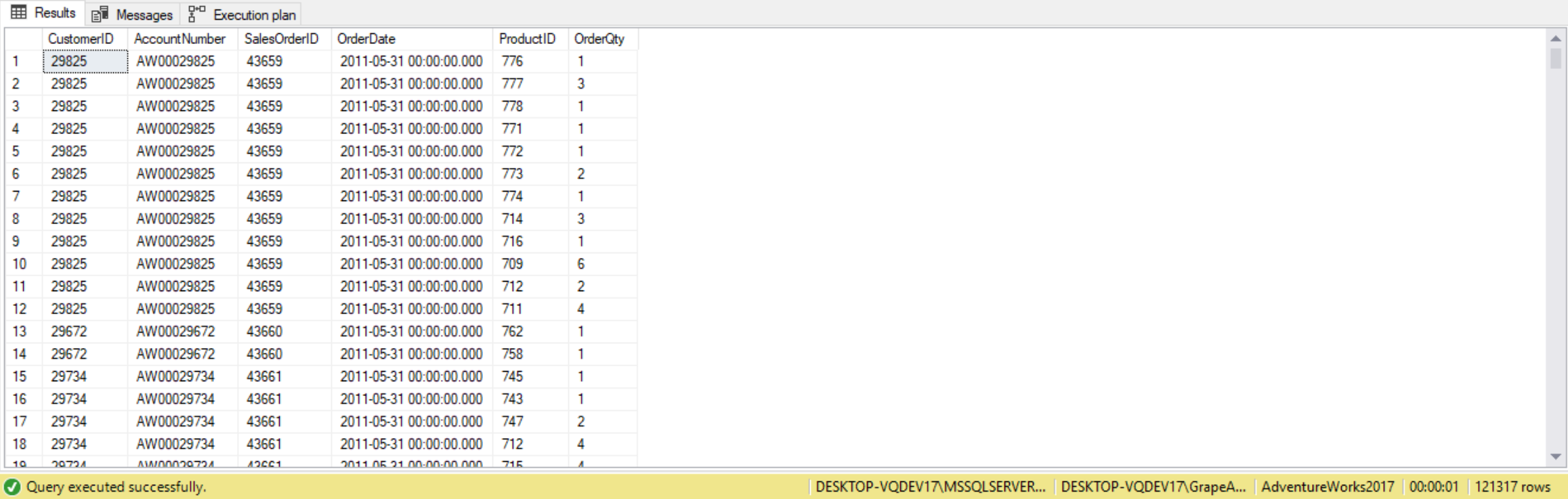
Adding a third table to an SQL-92 inner join requires adding another JOIN clause and another join condition in a separate ON clause.
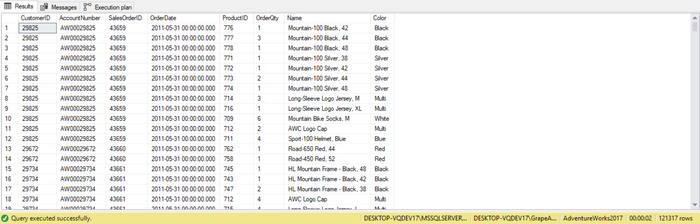
--Four table JOIN
SELECT c.CustomerID,
       c.AccountNumber,
       soh.SalesOrderID,
       soh.OrderDate,
       sod.ProductID,
       sod.OrderQty,
       p.Name,
       p.Color
FROM Sales.Customer AS c
     INNER JOIN Sales.SalesOrderHeader AS soh ON c.CustomerID = soh.CustomerID
     INNER JOIN Sales.SalesOrderDetail AS sod ON soh.SalesOrderID = sod.SalesOrderID
     INNER JOIN Production.Product AS p ON sod.ProductID = p.ProductID;
More join examples
Special use cases for joins include composite joins, non-equi joins, and multi-join queries.
Composite joins
A composite join is a join involving matching multiple attributes from each input table. These are typically used when a primary key-foreign key relationship is based on more than one attribute. For example, suppose we have a table dbo.Table2 that has a foreign key defined on columns col1 and col2, which references col1 and col2 of another table dbo.Table1. The FROM clause of the join query based on this relationship would be as follows:
(Include code, explanation, and results from page 135).
(Include a tangible example of composite joins from another source)
Non-equi joins
(Include notes from Joes2Pros, Udemy SQL, AbstractSQLEngineer, SQL Cookbook, Vertabelo Academy, 70-461 book, and Udemy ‘SQL Server Essentials’)
Any join involving use of the equality operator (=) is an equi join. A join that uses any operator besides the equality operator is a non-equi join. In other words, non-equi joins use comparison operators instead of equal (=).
For example, the following query joins two instances of the Employees table to return unique pairs of employees:
--Find all employees who have worked in more than one department
SELECT ed1.BusinessEntityID, --Employee
       ed2.BusinessEntityID
FROM HumanResources.EmployeeDepartmentHistory AS ed1
     JOIN HumanResources.EmployeeDepartmentHistory AS ed2 ON ed1.BusinessEntityID = ed2.BusinessEntityID
AND ed1.DepartmentID <> ed2.DepartmentID;
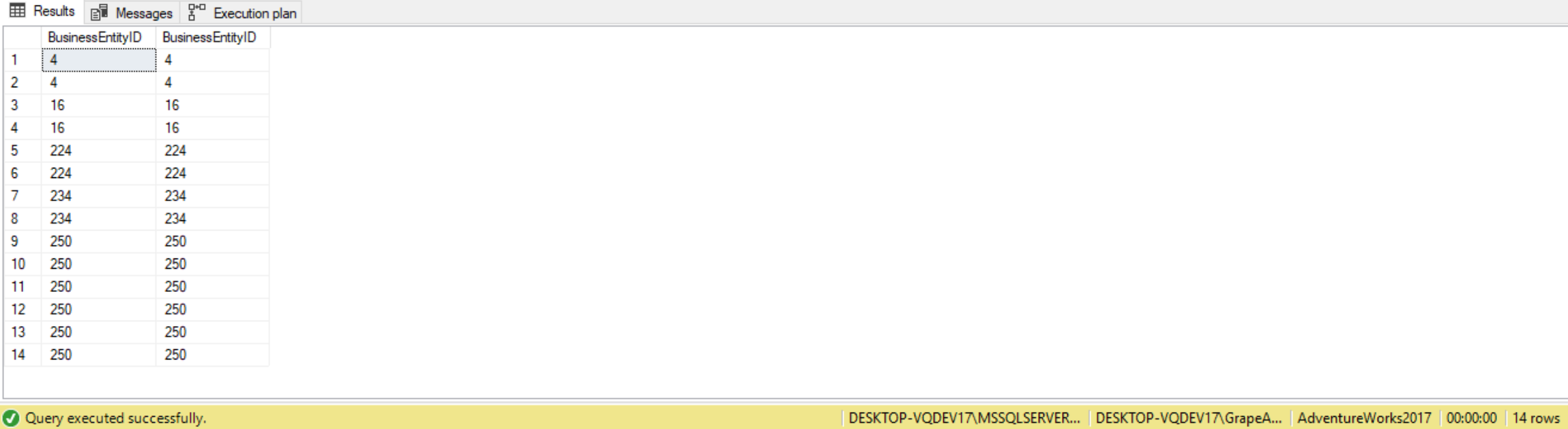
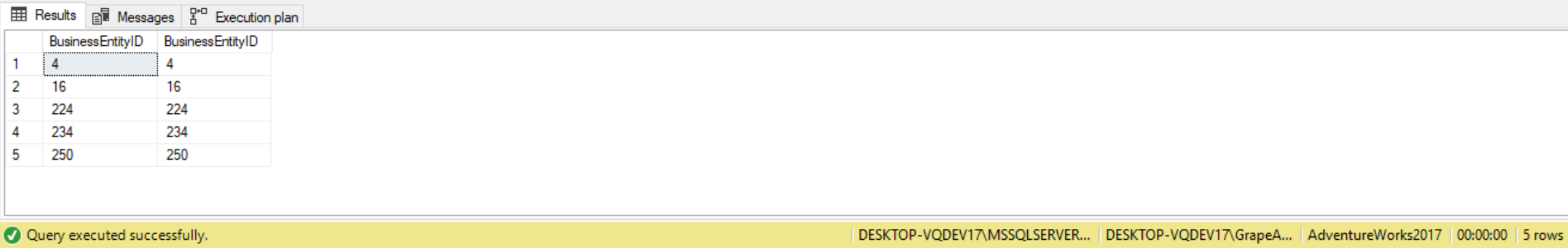
^^Employee 250 may have worked at the same department at two different times, hence the duplicate. To fix this, use the DISTINCT clause:
SELECT DISTINCT
       ed1.BusinessEntityID, --Employee
       ed2.BusinessEntityID
FROM HumanResources.EmployeeDepartmentHistory AS ed1
     JOIN HumanResources.EmployeeDepartmentHistory AS ed2 ON ed1.BusinessEntityID = ed2.BusinessEntityID
AND ed1.DepartmentID <> ed2.DepartmentID;
The non-equi inner join first produces a Cartesian product with the two Employee table instances, then filters the result set to return only records that are TRUE to the predicate e1.empid<e2.empid.
Common use cases for non-equi joins include generating pairs, calculating running totals and generating row numbers (prior to the introduction of window functions). Non-equi joins can also be used to check for duplicates or when we need to compare one value in a table falls within a range of values within one another.
Non-equi join to calculate running total
SET STATISTICS IO, TIME ON;

--Generate row numbers for the table using NON-EQUI join
SELECT soh1.CustomerID,
       soh1.SalesOrderID,
       COUNT(*) AS RowNumber
FROM Sales.SalesOrderHeader AS soh1
     --Row number based on how many rows soh1 is >= to soh2
     JOIN Sales.SalesOrderHeader AS soh2 ON soh1.SalesOrderID >= soh2.SalesOrderID
GROUP BY soh1.CustomerID,
         soh1.SalesOrderID
ORDER BY soh1.SalesOrderID;

--Performance comparison with equivalent ROW_NUMBER window function
SET STATISTICS IO,TIME ON;
SELECT CustomerID,
       SalesOrderID,
       ROW_NUMBER() OVER(ORDER BY SalesOrderID) AS RowNumber2
FROM Sales.SalesOrderHeader;
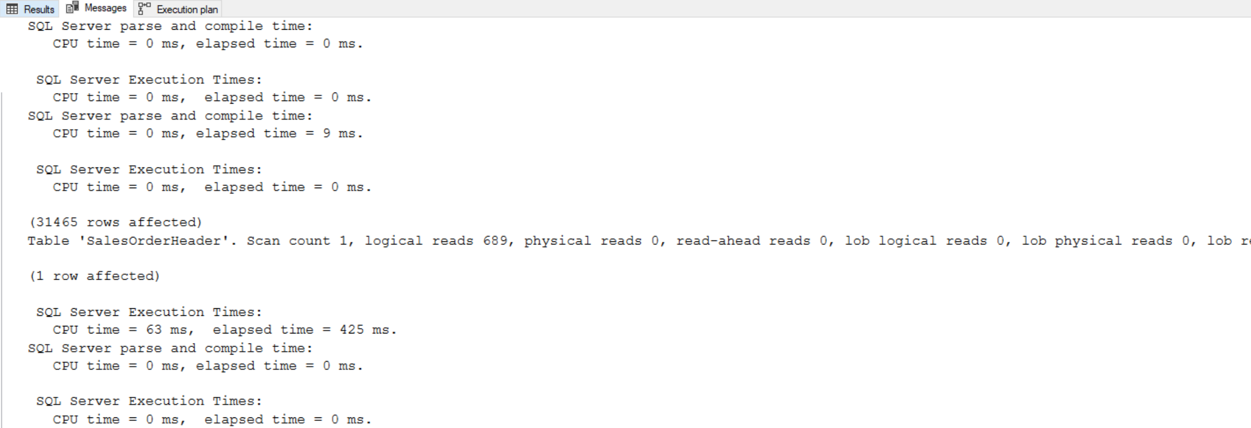
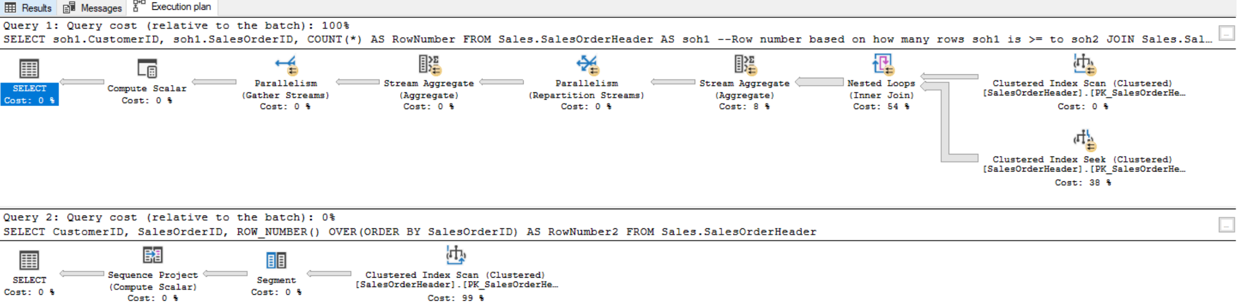
(Note the top execution plan is the query using the non-equi join, whereas the bottom execution plan is the query using the window function)
Notice that the first query took 37 seconds to return the complete result set. Comparison of the same query with an equivalent ROW_NUMBER window function shows that the ROW_NUMBER performs significantly better:
(Include image of execution plan, and explain how those two queries compare in terms of performance)
Non-Equi Join to check for duplicate values
In this example, we’ll be using the Person.Person table to look at first name and last name. We will be checking the table to see if there are any rows that have the same first name and last name across the table. The BusinessEntityID is the primary key, so that is unique. The query would go as follows:
SELECT P1.FirstName,
       P1.LastName,
       P1.Title,
       P1.MiddleName,
       P2.MiddleName,
       P2.Title
FROM Person.Person P1
INNER JOIN Person.Person P2 ON P1.FirstName = P2.FirstName
       AND P1.LastName = P2.LastName
       AND P1.BusinessEntityID <> P2.BusinessEntityID
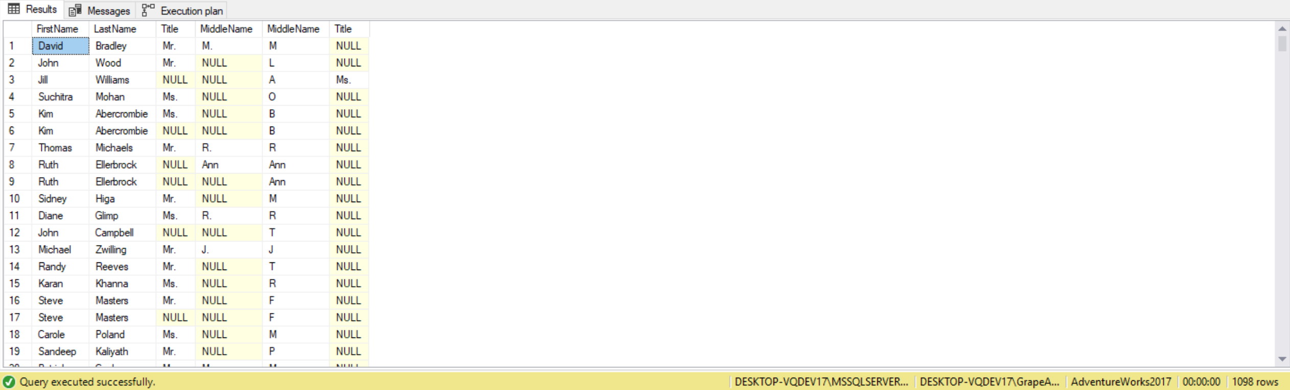
Here we are self-joining from the Person.Person table on FirstName and LastName. We’re also joining where the BusinessEntityID do not match to ensure the record is not a duplicate even though the first and last names match.
Compare a range of values using a non-equi join
(Update from Wenzel)
The Salary Levels Scenario
Here, we have another scenario that requires non-equal joins. Suppose we’re using the HumanResources database and we wish to retrieve employee and salary-level information.
The code to create our demo tables is as follows:
(Include the code to create the Employees table)
CREATE TABLE salarylevels
  (
     lowbound  DECIMAL(7, 2) NOT NULL,
     highbound DECIMAL(7, 2) NOT NULL,
     sallevel  VARCHAR(50) NOT NULL
  )

INSERT INTO salarylevels
VALUES     (0.00,
            1500.00,
            'Doing most of the work')

INSERT INTO salarylevels
VALUES     (1500.01,
            2500.00,
            'Planning the work')

INSERT INTO salarylevels
VALUES     (2500.01,
            4500.00,
            'Tell subordinates what to do')

INSERT INTO salarylevels
VALUES     (4500.01,
            99999.99,
            'Owners and their relatives')
Our query involves joining the Employees and SalaryLevels tables, as shown below:
SELECT E.*,
       sallevel
FROM   employees AS E
       JOIN salarylevels AS SL
         ON E.salary BETWEEN lowbound AND highbound
Multi-join queries
(MERGE WITH INNER JOIN SYNTAX)
Even though join operations are between two tables, a query can contain multiple joins. The join operators are logically processed from left to right. In other words, the result of the first join operation serves as the left table input for the second join, and the result of the second join operation serves as the left table input to the third join, and so on. Note that with cross joins and inner joins, the database engine can internally re-arrange the join ordering to optimize the query, but will still return the correct result set for the query.
For example, the following query joins the Customers and Orders tables to match customers with their orders, and joins the result of that to the OrderDetails table to match orders with their order lines:
(Include code, explanation, and results from page 138).
Outer joins
(Include notes from Joes2Pros, Udemy SQL, AbstractSQLEngineer, SQL Cookbook, Vertabelo Academy, 70-461 book, and Udemy ‘SQL Server Essentials’)
Fundamentals of outer joins
Outer join involves three logical querying processes: it first applies a Cartesian product between two input tables like a cross join or inner join, and then it filters the rows based on a specified predicate using the ON filter, and finally it adds outer rows.
- The LEFT JOIN will return all records from the first table (the table on the left side of the JOIN keyword), and also matching records from the second table (the table on the right side of the JOIN keyword). NULL is returned for any records from the first table having no matches from the second table.
- The RIGHT JOIN is similar to the LEFT JOIN, the only difference being that the tables are switched around. In other words, with a right join, all records from the second table (the table on the right side of the JOIN keyword) is returned, and also matching records from the first table (the table on the right side of the JOIN keyword). NULL is returned for any records from the second table having no matches from the first table.
- The FULL OUTER join will return all records from both tables. It’s essentially a combination of a LEFT JOIN and a RIGHT JOIN. If a match is found, then the matching records are returned, otherwise NULL is returned. It’s similar to a LEFT JOIN or RIGHT JOIN, but differs in that it looks for matches both ways and displays NULL in either set of data.
We can change a LEFT JOIN to a RIGHT JOIN (and vice versa) by swapping the join types or table names.
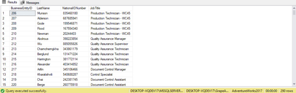
As an example, the following query uses a left join to list all Person.LastName and also the JobTitle if the person is an employee. We’re returning all records from the Person table, even records that don’t match the Employee table:
SELECT Person.Person.BusinessEntityID,
       Person.Person.LastName,
       HumanResources.Employee.NationalIDNumber,
       HumanResources.Employee.JobTitle
FROM   person.Person
LEFT OUTER JOIN
      HumanResources.Employee
      ON person.BusinessEntityID = Employee.BusinessEntityID;
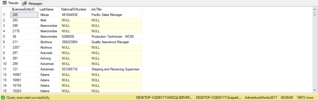
(Notice NULL is returned for NationalIDNumber and JobTitle for BusinessEntity ID 293. This is because there are no employees matching BusinessEntityID of 293.
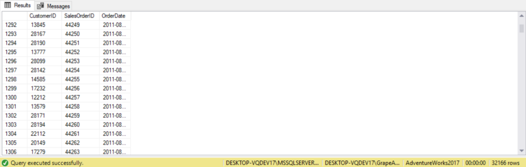
For example, to return employee and department information using the two-way left outer join, the query would be as follows:
--Entire list of customers regardless if they have a purchase or not
SELECT c.CustomerID,
       soh.SalesOrderID,
       soh.OrderDate
FROM Sales.Customer AS c
     LEFT JOIN Sales.SalesOrderHeader AS soh ON c.CustomerID = soh.CustomerID
ORDER BY soh.OrderDate;
More examples of a left outer join:
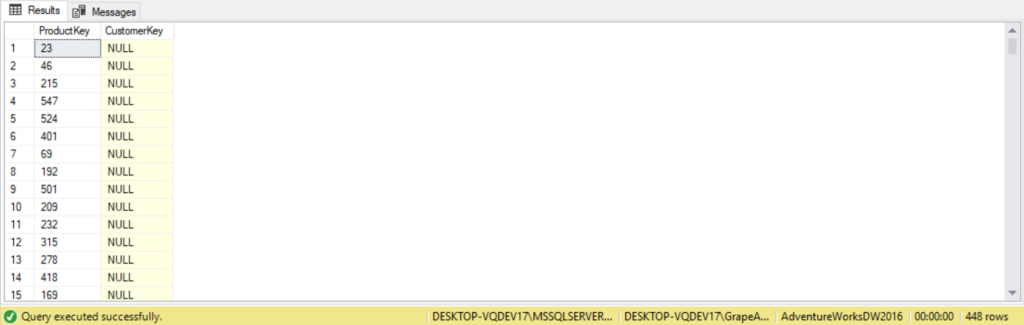
--Left Outer Join to find all Products on DimProduct not sold on FactInternetSales
--If fis.CustomerKey is NULL, then the ProductKey is not sold on FactInternetSales
USE AdventureWorksDW2016;
SELECT dp.ProductKey,
       fis.CustomerKey
FROM DimProduct AS dp
     LEFT JOIN FactInternetSales AS fis ON dp.ProductKey = fis.ProductKey
WHERE fis.CustomerKey IS NULL;
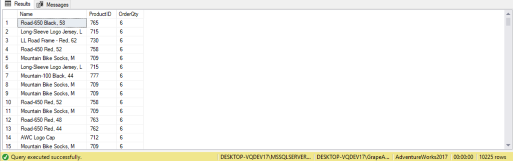
--List of all products and quantity sold where quantity sold is greater than 5
SELECT p.Name,
       p.ProductID,
       sod.OrderQty
FROM Production.Product AS p
     LEFT JOIN Sales.SalesOrderDetail AS sod ON p.ProductID = sod.ProductID
WHERE sod.OrderQty > 5
ORDER BY sod.OrderQty;
(Include code, explanation, and results from page 15 of ADVANCED BOOK).
The following query is an example of a right outer join. They key difference from the left outer join here is we’re returning all records from the Employee table, which is the table to the right of the JOIN keyword. If a matching employee record isn’t found, then NULL will be returned for BusinessEntityID and LastName.
SELECT Person.Person.BusinessEntityID,
       Person.Person.LastName,
       HumanResources.Employee.NationalIDNumber,
       HumanResources.Employee.JobTitle
FROM   Person.Person
RIGHT OUTER JOIN
      HumanResources.Employee
      ON person.BusinessEntityID = Employee.BusinessEntityID;
Note that no NULL is returned. This because there is a 0..1 to 1 relationship between Employee and Person. This means that for every Employee there is one Person, so in the case of a right join there won’t exist any non-matching rows. With this type of relationship, we could have also used an inner join.
(Include code, explanation, and results from page 16 of ADVANCED BOOK).
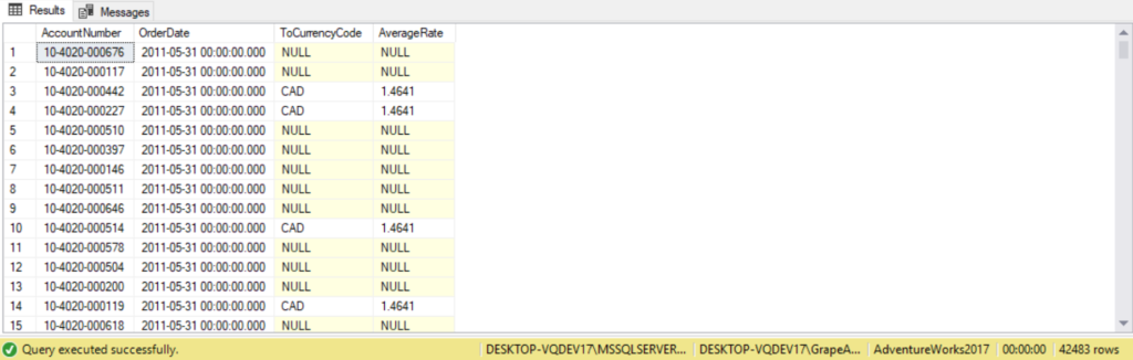
The following query uses a full outer join to return all the currencies we can place orders in and which orders were placed in those currencies.
SELECT Sales.SalesOrderHeader.AccountNumber,
       Sales.SalesOrderHeader.OrderDate,
       Sales.CurrencyRate.ToCurrencyCode,
       Sales.CurrencyRate.AverageRate
FROM   Sales.SalesOrderHeader
FULL OUTER JOIN
       Sales.CurrencyRate
       ON Sales.CurrencyRate.CurrencyRateID = Sales.SalesOrderHeader.CurrencyRateID;
(Include code, explanation, and results from page 17 of ADVANCED BOOK).
The above full outer query consists of 1.) All matching rows from both tables. 2.) All rows from the Employees tables with no matching department, with NULLs replacing the values that were supposed to come from the Departments table. 3.) All rows from the Departments table with no matching employee, with NULLS replacing the values that were supposed to come from the Employees table. With left and right outer joins, the order in which the tables appear in the query determines the order of their processing. This, of course, makes sense because their order affects the output. In the case of full outer joins however, their order doesn’t affect the output; hence, it doesn’t determine their processing order.
Outer joins enable us to define either one or both tables participating in the join as preserved tables. The third logical querying processing phase of the outer join identifies rows from the preserved table that have no matches in the other table on the ON predicate. This means that besides returning matching rows from both tables, the rows from the preserved table that have no match in the other table are also returned, padded with NULLs instead of the values that were supposed to come from the other table.
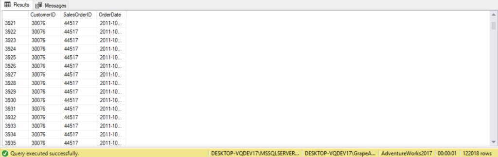
For example, the following query joins the Customers and Orders tables to return customers and their orders. In this case, all rows from the customers table are preserved. For customers with no orders, the query returns NULL for ordered:
SELECT c.CustomerID,
       soh.SalesOrderID,
       soh.OrderDate
FROM Sales.SalesOrderHeader AS soh
     RIGHT JOIN Sales.Customer AS c ON c.CustomerID = soh.CustomerID
ORDER BY soh.OrderDate;
As we can see customer ID 27 and 57 from the Customers table placed no orders, so the query returns NULL for orderid from the Orders table. The records for those two customer IDs were discarded by the second logical querying phase since there were no matching records on the Orders table, but the third logical querying phase added those two records back to the result set as outer rows. Those two rows were added back to preserve all rows of the left (Customers) table.
More examples:
--Three table outer JOIN using Customer, SalesOrderID, and SalesOrderHeader tables
SELECT c.CustomerID,
       soh.SalesOrderID,
       soh.OrderDate
FROM Sales.Customer AS c
     LEFT JOIN sales.SalesOrderHeader AS soh ON c.CustomerID = soh.CustomerID
     LEFT JOIN Sales.SalesOrderDetail AS sod ON soh.SalesOrderID = sod.SalesOrderID
ORDER BY soh.SalesOrderID;
There’s two kind of rows with respect to the preserved side when working with outer joins – inner and outer rows. Inner rows are those that have matches on the other table in the ON predicate, whereas outer rows don’t have matches. An inner join returns only inner rows, while an outer join returns both the inner and outer rows of the preserved table.
It’s important to distinguish between specifying the predicate in the ON or WHERE clause of query. Remember that the ON clause only determines whether a row will be matched with rows in the table on the other side of the ON clause. We can use the WHERE predicate when we need to apply a filter after producing the outer rows. Because the WHERE clause is processed after the FROM clause, this also means that it’s processed after all joins (including outer joins) are produced. So, the ON clause is used to specify matching (nonfinal) predicates, whereas the WHERE clause is used to specify a filtering (final) predicate.
Suppose we wish to return only outer rows, rows with no matches on the other table. We can update our previous query by adding a WHERE filter to return only those outer rows. Since the outer rows returns NULL on attributes from the nonpreserved table, we can simply filter for only rows that return NULL from the nonpreserved table, like the following query:
(Include code, explanation, and results from page 139).
Remember to always use IS NULL and not =NULL. This is because if we use the equality operator to compare values to a NULL, it always evaluates to UNKNOWN, even if we’re comparing two NULLs. There are three cases for selecting the ideal preserved attribute that can produce outer rows: a primary key column, a join column, and a column defined as NOT NULL. A primary key column and a column defined as NOT NULL cannot have NULL records, so a NULL returned from a nonpreserved table can only mean the row is an outer row. If a row has a NULL in the join column, that row is filtered out by the second phase of the join, so a NULL in such a column can only means that it’s an outer row.
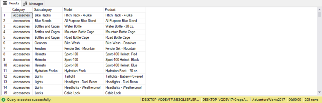
As an advanced example, let’s explore the production schema to produce a list of all product categories and the product models contained within. The Product table has a one to many relationship with ProductModel and ProductSubcategory. There is also an implicit many to many relationship between ProductModel and ProductSubcategory. Because of this, it is a good candidate for outer joins as there is may be a product models with no assigned products and ProductSubCategory entries with no product. To overcome this situation we do an outer join to both the ProductModel and ProductCategory table. The code would be as follows:
SELECT   PC.Name AS Category,
         PSC.Name AS Subcategory,
         PM.Name AS Model,
         P.Name AS Product
FROM     Production.Product AS P
FULL OUTER JOIN
         Production.ProductModel AS PM
         ON PM.ProductModelID = P.ProductModelID
FULL OUTER JOIN
         Production.ProductSubcategory AS PSC
         ON PSC.ProductSubcategoryID = P.ProductSubcategoryID
INNER JOIN
         Production.ProductCategory AS PC
         ON PC.ProductCategoryID = PSC.ProductCategoryID
ORDER BY PC.Name, PSC.Name
Beyond the fundamentals of outer joins
Including missing values
Because outer joins not only return matching rows but also those that don’t, can be used to identify and include missing values when querying data. For example, suppose we’re concerned that we may have some ProductSubcategory entries that don’t match to Categories. We can test this by running the following query:
SELECT PSC.Name AS Subcategory
FROM Production.ProductCategory AS PSC
     LEFT OUTER JOIN Production.ProductSubcategory AS PC
     ON PC.ProductCategoryID = PSC.ProductCategoryID
WHERE PSC.ProductCategoryID IS NULL;
The outer join returns the unmatched rows as NULLs. The WHERE clause filters on the non-NULL records, leaving only nonmatching Subcategory names for us to review.
Filtering attributes from the nonpreserved side of an outer join
If a predicate in the WHERE clause involves an attribute from the nonpreserved table using an expression in the form of <attribute><operator><value>, it’s usually an indication of a bug. This is because attributes from the nonpreserved table are NULLs in outer rows, and an expression in the form of NULL<operator><value> yields UNKNOWN unless we’re using the IS NULL operator. Remember the WHERE clause filters out records that evaluate to UNKNOWN. Such a predicate in the WHERE clause will filter out all outer rows, effectively turning the outer join into an inner join. So there’s a mistake in either the join type or the predicate. For example, let’s examine the following query:
(Include code, explanation, and results from page 143)
The above query applies a left outer join between the Customer and Order tables. The predicate o.orderdate>=’20160101’ in the WHERE clause evaluates for UNKNOWN for all the outer rows, because those records are NULL in the o.orderdate column. All other rows are discarded by the WHERE filter, as we see in the results.
As we can see, the outer join here was futile. There was either a mistake in using an outer join or specifying a predicate in the WHERE clause.
Using outer joins in a multi-join query
Table operators like joins are logically evaluated from left to right. Changing the order in which the outer join is processed may result in a different result set being returned.
There may be bugs that arise related to the logical order in which outer joins are processed. For example, suppose we have a query that involves an outer join between two tables, and then an inner join between the result and a third table. In the predicate on the inner join’s ON clause compares a column from the nonpreserved table of the outer join with a column from the third table, all outer rows from the outer join are discarded. Remember that outer joins have NULLs from the nonpreserved table and comparing NULLs with anything evaluates to UNKNOWN. Any record evaluating to UNKNOWN gets filtered out by the ON clause. In other words, such a predicate renders the outer join futile and effectively turns it into an inner join. For example, let’s examine the following query:
(Include code, explanation, and results from page 145)
The first join is an outer join that returns all customers and their orders as well as customers with no orders. The second join is an inner join that matches the result of the outer join with the OrderDetails table, based on the predicate o.orderid=od.orderid. For customers with no orders, the o.orderid is NULL, and therefore these records evaluate to UNKNOWN and are discarded. As we can see in the results, customers 22 and 55 did not place any orders, and are not included in the result set.
Generally, outer rows are discarded whenever an outer join (left, right, or full) is followed by a subsequent inner join or right outer join. Of course, this is assuming the join condition compares the NULLs from the left side with something from the right side.
An option to get around this issue is to use a left outer join as the second join as well, as shown below:
(Include code, explanation, and results from page 146)
As we can see, the outer rows from the first outer join are preserved, since we have both customer 22 and 57 returned.
This is not the best solution because it preserved all rows from the Orders table. If we want records from the Orders table having no matches to OrderDetails to be discarded, then we apply an inner join between Orders and OrderDetails.
A second solution is to apply an inner join between Orders and OrderDetails first, then use the result in a right outer join with the Customers table, as shown below:
(Include code, explanation, and results from page 146)
As we can see, the outer rows that resulted from right outer join are not filtered out.
A third solution would be to turn the inner join between Orders and OrderDetails into an independent unit by placing them inside paretheses. This way we can apply a left outer join between the result set from the operation inside the parentheses with the Customers table, as shown below:
(Include code, explanation, and results from page 147)
Using the COUNT aggregate with outer joins
Another common bug involves using COUNT with outer joins. When grouping the result of an outer join and using the COUNT(*) aggregate, the aggregate counts both inner and outer rows since it counts rows regardless of their contents. Typically, outer rows are not considered when counting. For example, the following query returns the count of orders for each customer
(Include code, explanation, and results from page 147)
Customer 22 and 57 have no orders but are still returned in the result of the join, and therefore show up in the out with a count of 1.
COUNT(*) doesn’t really detect whether a row really represents an order. To fix this issue, we should use COUNT(<column>) instead of COUNT(*) and provide a column from the nonpreserved table. This way, the COUNT() function ignores outer rows since they contain NULLs in the nonpreserved table column. We should use a column that can be NULL only when the rows is an outer row, for example the primary key column orderid:
(Include code, explanation, and results from page 148)
As we can now see, customers 22 and 57 have a count of 0.
Using JOINs to Modify Data
Sometimes we may need to modify data but the criteria that define which rows need to be affected is based on data that doesn’t exist in the modified table. Instead, the required data is another table. Besides the use of subqueries, we can accomplish this by using joins in the DELETE and UPDATE statements. Please note that the queries in this section are not ANSI compliant.
Using JOINS to delete data
Suppose we’re using the Northwind database, and we wish to delete all rows from the Order Details table for orders made by a customer ‘VINET.’ The problem is that the Order Details table does not hold the customer information. This information exists in the Orders table, so this is how the query would go:
(Include code, explanation, and result from page 43-44)
The first occurrence (after the first FROM clause) specified which table is modified, and the second occurrence (after the second FROM clause) is used for the join operation. This syntax doesn’t allow you to specify more than one table after the first FROM clause. If it did, it wouldn’t be possible to determine which table is modified.
Using JOINs to Update Data
The UPDATE statement has a similar syntax to the DELETE statement. Suppose we wish to add a 5 percent discount to items in the Order Details table whose parts are supplied by Exotic Liquids, SupplierID 1. The issue is that the SupplierID column is in the Products table, and we wish to update the Order Details table. Here is how we can write the update query:
(Include code, explanation, and result from page 44)
(Include OUTER JOIN in Data Warehousing example from PragmaticWorks Advanced JOIN course)
Performance Considerations
Here we discuss using hints to specify a certain join strategy and provide a few guidelines to help achieve better performance with our join queries.
Completely Qualified Filter Criteria
While it may seem obvious that if A=B and B=C then A=C, this is not as obvious to SQL Server’s optimizer. Let’s say we want a list of orders and their details for all orderIDs from 11,000 upward. We could filter the Orders table or the Order Details table, but if we apply the filter to both tables, there is far less I/O. Here is a query for an incompletely qualified filter criterion:
(Include code, explanation, and result from page 45)
Let’s revise this query so that it uses a completely qualified filter criteria, as shown below:
(Include code, explanation, and result from page 46)
Notice the significant difference in the number of logical reads required to satisfy the first query as opposed to the second one. Also, the first query plan uses a nested-loops join algorithm, and the second one uses the more efficient merge join algorithm.
Join Hints
As of SQL Server 2017, four join strategies are available: nested loops, hash match, merge join, and adaptive join. If we are testing the performance of our query, and would like to force a certain join algorithm, we can specify it by using a join hint, as shown below:
(Include code, explanation, and result from page 46)
The <join_hint> clause stands for LOOP, MERGE, or HASH. If we specify a join hint, specifying a join type becomes mandatory, and we cannot rely on defaults.
Performance Guidelines
The following can help achieve better performance for our join queries:
- Create indexes on frequently joined columns. Use the Index Tuning Wizard for recommendations.
- Create covering (composite) indexes on combinations of frequently fetched columns.
- Create indexes with care, especially covering indexes. Indexes improve the performance of SELECT queries but degrade the performance of modifications.
- Separate tables that participate in joins onto different disks by using filegroups to exploit parallel disk I/O.